Final exam
Prepare using:
# Case links:
"""
Yeah I know, this does not run on Colab. :)
The solution requires web scraping or the GitHub Python API.
If you have a better solution, let me know.
"""
import os

for file in os.listdir('cases'):
    if file.endswith("ipynb"):
        print('https://colab.research.google.com/github/cafawo/Derivatives/blob/main/cases/' + file)
https://colab.research.google.com/github/cafawo/Derivatives/blob/main/cases/1_warmup.ipynb
https://colab.research.google.com/github/cafawo/Derivatives/blob/main/cases/1_warmup_solutions.ipynb
https://colab.research.google.com/github/cafawo/Derivatives/blob/main/cases/2_forward.ipynb
https://colab.research.google.com/github/cafawo/Derivatives/blob/main/cases/2_forward_solutions.ipynb
https://colab.research.google.com/github/cafawo/Derivatives/blob/main/cases/3_fixedincome.ipynb
https://colab.research.google.com/github/cafawo/Derivatives/blob/main/cases/3_fixedincome_solutions.ipynb
https://colab.research.google.com/github/cafawo/Derivatives/blob/main/cases/4_bund.ipynb
https://colab.research.google.com/github/cafawo/Derivatives/blob/main/cases/4_bund_solutions.ipynb
https://colab.research.google.com/github/cafawo/Derivatives/blob/main/cases/5_options.ipynb
https://colab.research.google.com/github/cafawo/Derivatives/blob/main/cases/5_options_solutions.ipynb
https://colab.research.google.com/github/cafawo/Derivatives/blob/main/cases/6_credit.ipynb
https://colab.research.google.com/github/cafawo/Derivatives/blob/main/cases/6_credit_solutions.ipynb
https://colab.research.google.com/github/cafawo/Derivatives/blob/main/cases/_template.ipynb
Reading:
A financial derivative is a financial instrument whose value is derived from the value of another underlying asset, index, rate, or financial instrument. Derivatives can be used for various purposes including hedging risk, speculating on future prices, and gaining exposure to an asset class without having to own the underlying assets.
Consider, as a simple example, the forward contract, which is an agreement to exchange some underlying asset $S$ for price $K$ at some future point in time $T$, the cash flow of this derivative can therefore be written as
$$S_T - K$$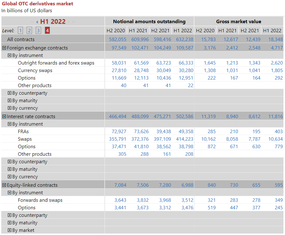
(Source: Bank for International Settlements, 2022)
For reference, the US GDP was 23.32 trillion USD in 2021.
Put-Call-Parity is the arbitrage relationship between (European) put, call, and forward.
$$PV(\text{Call}) - PV(\text{Put}) = S_0 - PV(K)$$With cash flows at maturity $T$:
$$\text{Call}_{T} = max(S_T - K, 0) = (S_T - K)^+$$$$\text{Put}_{T} = max(K - S_T, 0) = (K - S_T)^+$$$$\text{Forward}_{T} = S_T - K$$For example, if a call option is overpriced w.r.t. its replicating portfolio, i.e. Fwd + Put, sell the call and buy the replication. The resulting shift in supply and demand must adjust prices.
"""Spot price vs cash flow (put-call parity)
"""
import numpy as np
import matplotlib.pyplot as plt

S_T = np.linspace(0,100)
K = 50

# portfolio
CF_T = - np.maximum(K - S_T, 0) + np.maximum(S_T - K, 0)
#CF2_T = np.maximum(S_T - K, 0)

# the rest is plotting
plt.figure('PCP', figsize=(9,4))
plt.plot(S_T, CF_T)
#plt.plot(S_T, CF2_T)
plt.axhline(y=0, linewidth=1, color="black")
plt.xlabel("Spot price")
plt.ylabel("Cash flow")
plt.annotate("K", (K,-5))
plt.show()

... or can financial engineering cure cancer? (Fagnan, D. E., Fernandez, J. M., Lo, A. W., & Stein, R. M. (2013). Can financial engineering cure cancer?. American Economic Review, 103(3), 406-411.)

Interest rates are quoted per annum (p.a.) but speak different “languages”:
Money Market (MM):
$C_0(1+r_{mm}T_{mm})=C_T$
ISMA (International Securities Market Association - Europe)
$C_0(1+r_{isma})^T=C_T$
SIA (Securities Industry Association - US)
$C_0(1+r_{sia}/2)^{2T}=C_T$
Continous compounding (academia, financial engineering)
$C_0 e^{rT} = C_T$
$T$ is calculated by dividing the number of days in perid T by a year basis, e.g.
$T = act/360$ (Money Markets - DE/US/...)
$T = act/act$ (Bond - ISMA)
$T = 30/360$ (Swap)
These are some examples for day count conventions, which might differ from country to country. Observe that for $act/act$ and $30/360$, a full year must always yield $T=1$.
"""Interest rate conversion (translation)
"""
import numpy as np

r_isma = 0.1
r_mm = (r_isma*360/365)
r_sia = ((1+r_isma)**0.5-1)*2
r_cont = np.log(1+r_isma)

print(f'r_isma  = {r_isma:.4f}')
print(f'r_mm    = {r_mm:.4f}')
print(f'r_sia   = {r_sia:.4f}')
print(f'r_cont  = {r_cont:.4f}')
r_isma  = 0.1000
r_mm    = 0.0986
r_sia   = 0.0976
r_cont  = 0.0953
Semi-annual compounding has value only for didactical puposes, this is, when increasing the number of compounding periods $m$
$$C_0 \left( 1+\frac{r}{m} \right)^{mT}=C_T$$"""Continous compounding
"""
import numpy as np
import matplotlib.pyplot as plt
def FV(m):
PV = 1
r = 1
T = 1
return PV * (1 + r / m)**(T * m)
#FV_m = list(map(lambda m: FV(m), range(1,250)))
FV_m = FV(np.arange(1,250))
# plotting
plt.figure('exp', figsize=(9,4))
plt.plot(FV_m)
plt.axhline(y=np.exp(1), linewidth=1, color="red")
plt.xlabel("m")
plt.ylabel("FV")
plt.show()
print(f'FV(m = 100000) = {FV(100000):.4f}')
print(f'EXP(1) = {np.exp(1):.4f}')

FV(m = 100000) = 2.7183
EXP(1)         = 2.7183

# Constants
num_days = 31
annual_rate = 0.05

# GEnerate random path for S
np.random.seed(42)
noise = np.random.normal(loc=0, scale=1, size=num_days)
S = np.cumsum(noise) + 100

# Calculate the corresponding forward prices (F)
T = np.linspace(1, 0, num_days)  # Remaining maturity
F = S * np.exp(annual_rate * T)  # Forward price

# Plotting the smoother underlying and the forward for 30 days
plt.figure('spotfwd', figsize=(9,4))
plt.plot(S, label='Underlying (S)')
plt.scatter(0, S[0])
plt.plot(F, label='Forward (F)')
plt.scatter(0, F[0])
# Some additional markets and annotation
plt.axhline(y=F[0], color='gray', linestyle='--', label=r'Initial forward price ($F_0$)')
plt.annotate('', xy=(num_days-1, F[0]), xytext=(num_days-1, F[-1]), arrowprops=dict(arrowstyle="<->", color='green'))
plt.annotate(r'$S_T - K = F_T - F_0$', (num_days-1, (F[0]+F[-1])/2), ha='right', va='center', color='green', rotation=90)
# Labels and legend
plt.title('Spot vs forward until maturity (textbook)')
plt.xlabel('Days')
plt.ylabel('Price')
plt.legend()
plt.show()

To replicate a forward consider a portfolio that consists of underlying $S$ and cash $K$, which today is worth
$$f_0 = S_0 - K e^{-rT}$$and at maturity $T$
$$f_T = S_T - K$$The forward rate $F$ at initiation is set such that $f_0 = 0$, hence,
$$S_0 - F e^{-rt} = 0 \Leftrightarrow F = S_0 e^{rT}$$For many assets, additional factors affect the forward price, such as:
Considering all factors, we have
$$f_0 = S_0 e^{(-q-y+u)T} - K e^{-rT}$$and
$$F = S_0 e^{(r-q+u-y)T}$$"""Forward valuation
"""
def forward_price(spot, maturity, rate, income=0, storage=0, convenience=0):
return spot * np.exp((rate - income + storage - convenience) * maturity)
def forward_mtm(strike, spot, maturity, rate, income=0, storage=0, convenience=0):
return spot * np.exp((- income + storage - convenience) * maturity) - strike * np.exp(- rate * maturity)
# 12
print(f'E12: forward_mtm(55, 60, 1/2, 0.04) = {forward_mtm(55, 60, 1/2, 0.04):.2f}')
# 14
print(f'E14: forward_mtm(27, 25, 6/12, 0.1, 0.04) = {forward_mtm(27, 25, 6/12, 0.1, 0.04):.2f}')
print(f'E14: forward_price(25, 6/12, 0.1, 0.04) = {forward_price(25, 6/12, 0.1, 0.04):.2f}')
E12: forward_mtm(55, 60, 1/2, 0.04)       =  6.09
E14: forward_mtm(27, 25, 6/12, 0.1, 0.04) = -1.18
E14: forward_price(25, 6/12, 0.1, 0.04)   = 25.76
The risk of imperfect hedging.
Consider a long position in a risky asset $S$ to be hedged by selling (short) future $F$. We will hedge the asset in $t=1$, close the hedge in $t=2$ and analyze the basis $b$:
$b_1 := S_1 - F_1$
$b_2 := S_2 - F_2$
Value of the portfolio in $t=2$
$S_2 + F_1 - F_2 = \underbrace{F_1 + b_2}_{b_2 = S_2 - F_2}$
$b_2$ is unknown in $t=1$, hence, risky. Now also consider the underlying of the future $S^*$
$S_2 + F_1 - F_2 = F_1 + \underbrace{(S^*_2 - F_2)}_\text{time basis} + \underbrace{(S_2 - S^*_2)}_\text{underlying basis} \hspace{1cm} | S^*_2 - S^*_2 $
Reasons for basis risk:
"""Optimal hedge ratio vs linear regression beta
"""
import numpy as np
from numpy.random import randn
from numpy.polynomial.polynomial import polyfit
from scipy.linalg import cholesky
import matplotlib.pyplot as plt

corr = np.array([[1,.75],[.75,1]])
F, S = np.dot(randn(1000,2), cholesky(corr)).T
F = F * 2  # Assume that the future is about twice as volatile as the asset
constant, beta = polyfit(F, S, 1)

plt.figure('mvhegde')
plt.xlabel('Future (F)')
plt.ylabel('Asset (S)')
plt.scatter(F, S)
plt.plot(F, constant + beta * F, 'r-')
plt.show()

Hedge ratio for hedging asset S with future F
$$Var = \sigma^2_S + h^2\sigma^2_F-2 h \rho \sigma_S \sigma_F$$$$\frac{\delta Var}{\delta h} = 2 h \sigma^2_F - 2 \rho \sigma_S \sigma_F = 0$$$$...$$$$h = \rho \frac{\sigma_S}{\sigma_F}$$rho = np.corrcoef(F,S)[0][1]
sd_F = np.std(F)
sd_S = np.std(S)
print(f"rho(F,S) = {rho:.2f}")
print(f"Linear regression beta: {beta:.4f}")
print(f"Optimal hedge ratio h : {(rho*sd_S/sd_F):.4f}")
rho(F,S) = 0.76
Linear regression beta: 0.3686
Optimal hedge ratio h : 0.3686
A discount factor is today's price for 1 monetary unit in t, hence, a zero bond with face value 1 and maturity t.
$$C_0 = C_t DF_t \implies DF_t = \frac{C_0}{C_t}$$The discount factor does not "speak an interest rate language"! However, it can be translated into any interest rate convention, e.g.
$$C_0 = C_t \frac{1}{(1 + r)^t} \implies DF_t = \frac{1}{(1+r)^t} \implies r = \left(\frac{1}{DF_t}\right)^{1/t} - 1$$And as usual
$$PV = \sum^{T}_{t=1}\frac{C_t}{(1+r_t)^t} = \sum^{T}_{t=1}C_t DF_t$$"""Discounting for plain vanilla coupon bonds
"""
discount_factors = [.90, .80, .70]
def fair_price(coupon):
# sum(discount_factors) is an annuity factor
# the last discount factor [-1] discounts the face value
p = coupon * sum(discount_factors) + discount_factors[-1]
return p
print(f'Fair price 7% 3Y bond: {fair_price(0.07)*100:.4f}')
print(f'Fair price 10% 3Y bond: {fair_price(0.1)*100:.4f}')
print(f'Fair price 14% 3Y bond: {fair_price(0.14)*100:.4f}')
Fair price  7% 3Y bond:  86.8000
Fair price 10% 3Y bond:  94.0000
Fair price 14% 3Y bond: 103.6000
"""Coupon (nominal yield) vs yield to maturity
"""
from scipy.optimize import minimize
import matplotlib.pyplot as plt

discount_factors = [.9091, .8116, .7118]  # normal term structure
discount_factors = [.90, .80, .70]  # normal term structure
#discount_factors = [1/(1.12), 1/(1.10)**2, 1/(1.08)**3]  # inverted term structure


zero_rates = []
for T, DF_T in enumerate(discount_factors):
    T = T + 1
    r_T = (1 / DF_T) ** (1 / T) - 1
    zero_rates.append(r_T)
print([f"{r*100:.2f}%" for r in zero_rates])


# face value = 1!
def IRR_coupon(coupon, discount_factors):
    # calculate PV from market prices
    def fair_price(coupon):
        p = coupon * sum(discount_factors) + discount_factors[-1]
        return p
    # calculate PV from irr
    def IRR_price(irr, coupon):
        T = len(discount_factors)
        annuity_factor = (1 - (1 + irr) ** -T) / irr
        p = coupon * annuity_factor + 1 / (1 + irr) ** T
        return p
    # target function to be minimized
    def NPV2(irr):
        return (fair_price(coupon) - IRR_price(irr, coupon)) ** 2
    # set NPV = 0 and return both PVs and the irr
    opt = minimize(NPV2, x0=0.01, bounds = ((None, None),))
    return [fair_price(coupon), IRR_price(opt.x[0], coupon), opt.x[0]]


#print(IRR(.1, discount_factors))

# lets plot different coupon rates against their irr
x_coupons = range(100)
y_irrs = list(map(lambda c: IRR_coupon(c/100, discount_factors)[2]*100, x_coupons))

plt.plot(x_coupons, y_irrs)
plt.axhline(y=zero_rates[-1]*100, linestyle='--', linewidth=1, color='grey')
plt.xlabel("Coupon rate in %")
plt.ylabel("YTM (IRR) in %")
plt.show()
['11.11%', '11.80%', '12.62%']

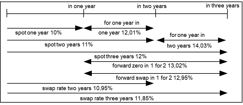
Forward rate fixed in $s$ payed in $t$ has arbitrage condition
$$(1+r_s)^s(1+r_{st})^{t-s} = (1+r_t)^t$$$$r_{st} = \left(\frac{(1+r_t)^t}{(1+r_s)^s}\right)^{1/(t-s)}-1$$Again, a discount factor $DF_t$ is today's value of 1 that is paid in $t$. Conversely, $1 / DF_t$ is a future value. This allows us to calculate "forward discount factors" by discounting $DF_t$ and compounding a shorter period $s$ with $1/DF_s$. Discounting with a forward discount factor or a forward rate must yield the same, hence,
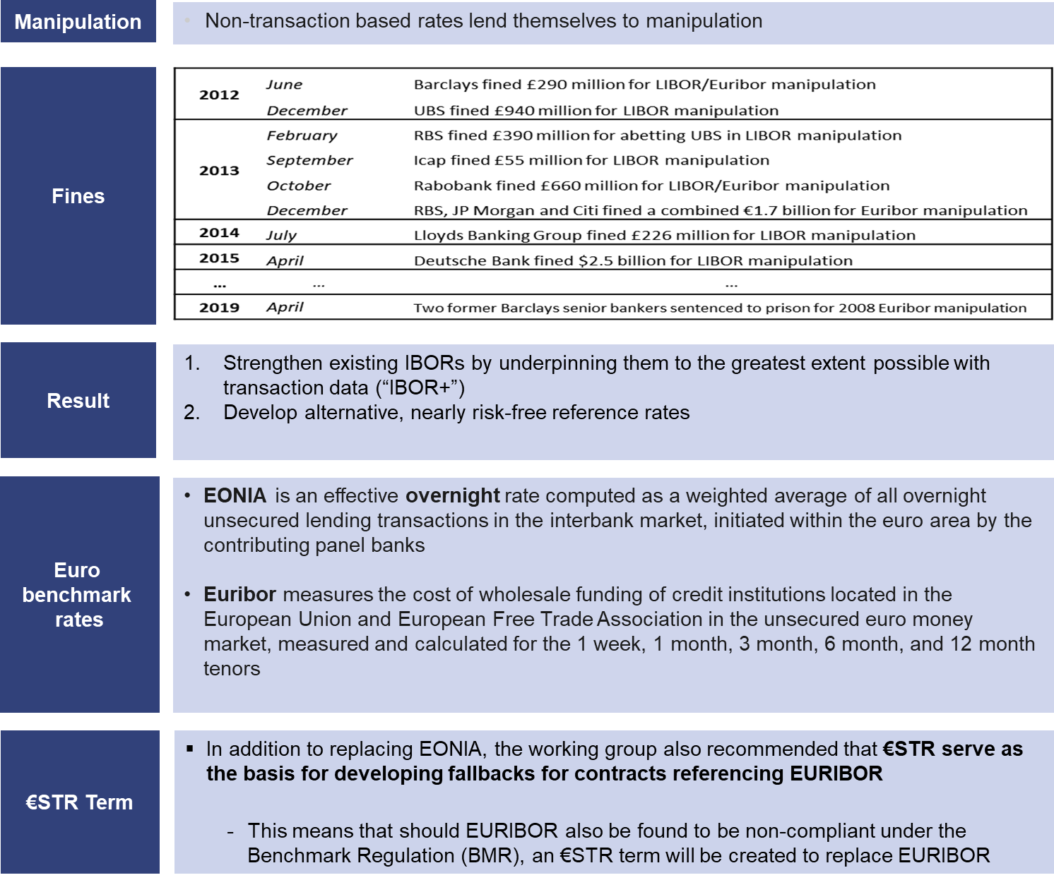
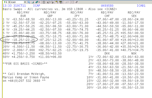
$$\begin{aligned} \frac{DF_t}{DF_s} &= \frac{1}{(1 + r_{st})^{t-s}}\\ &... \\ r_{st} &= \left(\frac{DF_s}{DF_t}\right)^{1/(t-s)}-1\\ &= \left(\frac{(1+r_t)^t}{(1+r_s)^s}\right)^{1/(t-s)}-1 \end{aligned}$$IBOR (Interbank Offered Rates) are a series of benchmark interest rates that represent the average interest rate at which a selection of banks are willing to lend to one another on an unsecured basis in the wholesale money market. The most popular IBORs are LIBOR (London Interbank Offered Rate), EURIBOR (Euro Interbank Offered Rate), and TIBOR (Tokyo Interbank Offered Rate). Reference rates are essential for many financial products, such as floating rate notes (FRN or floater). In an FRN, the IBOR rate $L_t$ is payed as a variable cash flow, hence,
$$ \begin{aligned} \text{PV}_\text{FRN} &= \sum_{t=1}^T L_t DF_t + DF_T \end{aligned} $$(Careful, this solution to the floater assumes that the next payment has just been fixed and that there has been no changes to the credit risk of the company.)
IBOR rates are quoted for various tenors, including overnight, one week, one month, three months, six months, and one year. Here is an example:
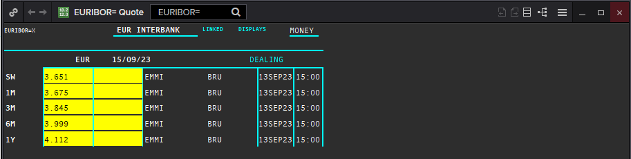
IBOR rates are typically quoted in accordance with the "actual/360" day count convention, though some variations like "actual/365" can also be observed depending on the currency and the specific IBOR.
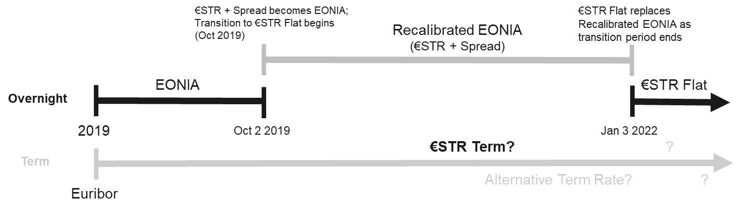
It's essential to note that, due to a series of scandals and a lack of underlying transactions to support the rates, the process of phasing out many IBORs, including LIBOR, started around 2020, with many countries transitioning to alternative reference rates (like SOFR in the USA, SONIA in the UK).
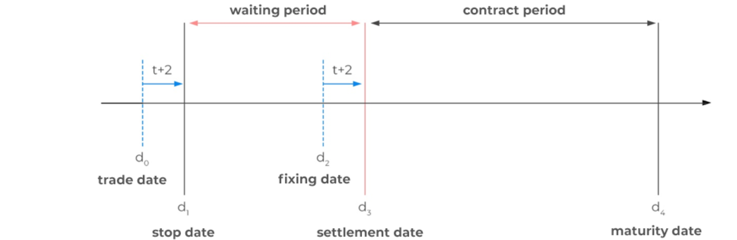
A Forward Rate Agreement (or FRA) is an agreement between two parties to exchange a short term underlying interest rate in the future.
$$\text{Settlement amount} = \frac{(L(d_2)-r(d_3,d_4)) \frac{act}{360}}{\left(1+L(d_2) \frac{act}{360}\right)} \times \pm \text{Nominal}$$A buyer enters into the contract to protect himself from increasing interest rates, hence, $+ \rightarrow$ buyer, $- \rightarrow$ seller.
Reading:
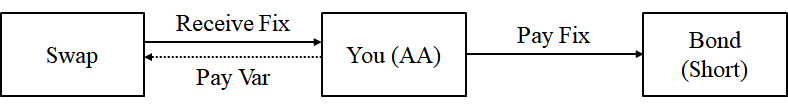
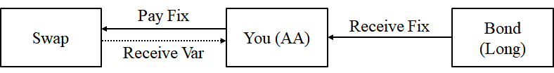
An interest rate swap is a financial derivative contract where two parties agree to exchange interest rate payments over a specified time period. Typically, one party pays a fixed interest rate, and the other pays a floating interest rate, which is usually tied to a benchmark rate such as EURIBOR. This contract allows parties to hedge risk or potentially benefit from changing interest rates.
def YTM(price, coupon, maturity):
    # calculate PV from irr
    def YTM_price(irr, coupon, maturity):
        T = maturity
        annuity_factor = (1 - (1 + irr) ** -T) / irr
        p = coupon * annuity_factor + 1 / (1 + irr) ** T
        return p
    # target function to be minimized
    def NPV2(irr):
        return (price - YTM_price(irr, coupon, maturity)) ** 2
    # set NPV = 0 and return both PVs and the irr
    opt = minimize(NPV2, x0=0.01, bounds = ((None, None),))
    return opt.x[0]

ytm_21 = YTM(100.5/100, 2/100, 5)
print(f'YTM = {ytm_21 * 100:.2f}%')
#print(f'Liability swap level = Euribor {(ytm_21 - 0.02) * 10000:.0f} basis points')

ytm_22 = YTM(101.0/100, 3/100, 5)
print(f'YTM = {ytm_22 * 100:.2f}%')
#print(f'Asset swap level = Euribor {(ytm_22 - 0.0205) * 10000:.0f} basis points')
YTM = 1.89%
YTM = 2.78%
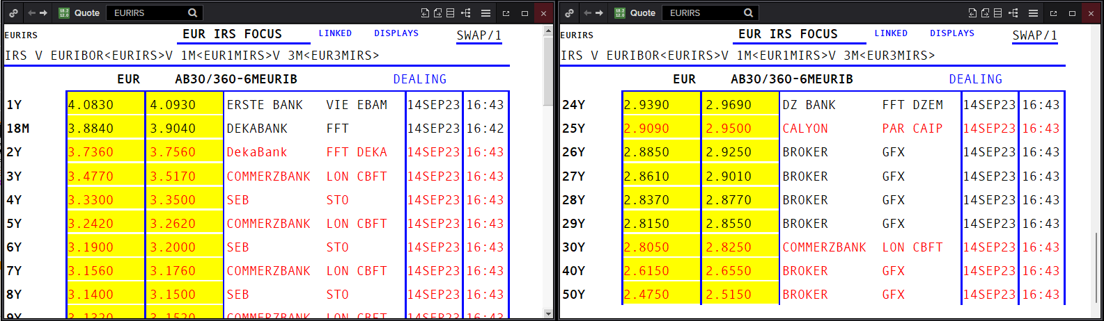
An interest rate swap (IRS) is the agreement to exchange a fixed ($C$) against a variable ($L_t$) payment. There exists a liquid market for swaps with maturities from 1 up to 50 years. For plain vanilla IRS we quote the fixed leg $C$. Note that the following swap quotes are all against 6M EURIBOR:
Assuming annual payments, we have
$$\begin{aligned} PV(Fix) &= C \sum_{t=1}^T DF_t\\ PV(Var) &= \sum_{t=1}^T L_t DF_t\\ &= \sum_{t=1}^T \left(\frac{DF_{t-1}}{DF_t} -1 \right) DF_t\\ &= 1 - DF_T \end{aligned}$$Price the fair swap rate $C$, such that,
$$\begin{aligned} PV(Fix) &= PV(Var)\\ C \sum_{t=1}^T DF_t &= 1 - DF_T\\ C &= \frac{1 - DF_T}{\sum_{t=1}^T DF_t} \end{aligned}$$Mark to market an existing swap with $C^*$ (the old swap rate) by comparing $PV(Fix)$ and $PV(Var)$
$$\begin{aligned} PV(Receiver) &= PV(Fix) - PV(Var)\\ &= C^* \sum_{t=1}^T DF_t - (1 - DF_T) \\ &= (C^* - C) \sum_{t=1}^T DF_t \end{aligned}$$Swap rate $C$ is also the par coupon bond rate that fulfills
$$\begin{aligned} 1 &= \sum^{T}_{t=1}C_t DF_t\\ &= C \sum^{T}_{t=1}DF_t + DF_T \implies C = \frac{1 - DF_T}{\sum^{T}_{t=1}DF_t} \end{aligned}$$Bootstrapping, i.e. creating zero bonds from a market of coupon bearing instruments
$$DF_t = \frac{1 - C_t \sum_{i=1}^{t-1} DF_i}{1 + C_t}$$"""Bootstrapping from swap rates (assuming annual payments)
"""
def swap_bootstrap(swap_rates):
discount_factors = []
for s in swap_rates:
# See Slide 61
DF_T = (1 - s * sum(discount_factors)) / (1 + s)
discount_factors.append(DF_T)
zero_rates = []
for T, DF_T in enumerate(discount_factors):
# Python starts counting at 0, hence, +1
T = T + 1
# See Slide 48
r_T = (1 / DF_T)**(1 / T) - 1
zero_rates.append(round(r_T,4))
return [discount_factors, zero_rates]
example = swap_bootstrap([0.04, 0.05, 0.06])
print(example)
[[0.9615384615384615, 0.9065934065934065, 0.8376529131246111], [0.04, 0.0503, 0.0608]]
"""Single curve swap pricing
"""
discount_factors = swap_bootstrap([0.04, 0.05, 0.06])[0]

def swap_pricing(discount_factors):
    # See Slide 66
    s_T = (1 - discount_factors[-1]) / sum(discount_factors)
    return s_T

print(f"3Y swap rate = {swap_pricing(discount_factors)*100:.2f}%")
3Y swap rate = 6.00%
"""Single curve forward swap pricing
"""
discount_factors = swap_bootstrap([0.04, 0.05, 0.06])[0]

# Please note that discount_factors is a vector that starts with the first discount factor (t = 1)
s_13 = (discount_factors[0] - discount_factors[-1]) / sum(discount_factors[1::])

print(f"1X2 swap rate = {s_13*100:.2f}%")
1X2 swap rate = 7.10%
Since the financial crisis, there exists a considerable spread between 6M Euribor and 6M Eonia Swap
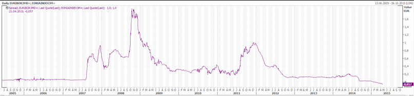
Since there exists a basis, it can be traded (basis swap).
It must still hold that
$$PV(\text{Fix}) =PV(\text{Var}),$$however, now, using different discount factors (from the Eonia curve), we need to find the relevant forward rates somewhere else. This is, we extract implied forward rates $\tilde{L}_t$ from a market of fair swap rates $C_T$, thus,
and hence,
$$\tilde{L_T} = \frac{C_T \sum_{t=1}^T DF_t - \sum_{t=1}^{T-1} \tilde{L_t} DF_t}{DF_T} \equiv \frac{CD - LD}{DF_T}.$$"""Calculate implied forward rates (multi curve approach)
"""
def multi_curve(swap_rates, eonia_rates):
# bootstrap discount factors from eonia rates
discount_factors = swap_bootstrap(eonia_rates)[0]
# setup
SDF = 0 # sum of discount factors
CD = 0 # discounted fixed leg until T
LD = 0 # discounted float leg until T-1
implied_forwards = []
for C_T, DF_T in zip(swap_rates, discount_factors):
SDF += DF_T # add up discount factors
CD = C_T * SDF # C_T is an annuity
L = (CD - LD) / DF_T # calculate implied forward rate (see equation above)
implied_forwards.append(round(L,4)) # round and save L
LD += L * DF_T # sum up discounted L (used in next iteration)
return implied_forwards
print(f"Implied forward rates: {multi_curve([0.04, 0.05, 0.06], [0.033, 0.045, 0.053])}")
Implied forward rates: [0.04, 0.0606, 0.082]
"""Price a forward swap (multi curve approach)
"""
implied_forwards = multi_curve([0.04, 0.05, 0.06], [0.033, 0.045, 0.053])
eonia_discount_factors = swap_bootstrap([0.033, 0.045, 0.053])[0]

PV_Var = sum(np.array(implied_forwards[1::]) * np.array(eonia_discount_factors[1::]))

s_13m = PV_Var / sum(eonia_discount_factors[1::])

print(f"1X2 swap rate (multi curve) = {s_13m*100:.2f}%")
1X2 swap rate (multi curve) = 7.09%
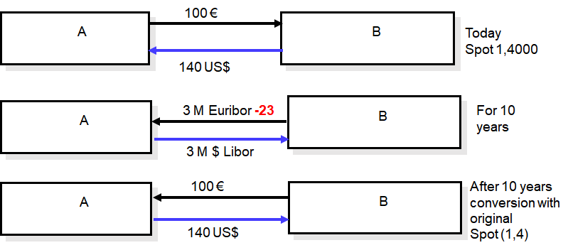
Let us start with two definitions:
The FX swap is an agreement to exchange spot at $S$ as well as in the future at forward rate $F_T$. According to Covered Interest Rate Parity, this has arbitrage relationship:
$$ \begin{align*} (1 + r_B \times T_B) F_T &= S (1 + r_Q \times T_Q) \\ &...\\ F_T &= S \frac{(1 + r_Q \times T_Q)}{(1 + r_B \times T_B)} \end{align*} $$By convention, FX forwards (aka FX ourights) are often quotet in FX swap points, this is,
$$\text{FX swap points} = F_T - S$$The FX swap market includes besides the interest rate differential also liquidity and credit advantages of the two currencies. Since the financial crisis the interest differential (interest rate parity) is not a good indicator for the FX swap anymore.

# FX outright
r_EUR = 1.43750 / 100
r_USD = 1.05310 / 100
EURUSD = 1.3193
T_act = 365

FX_Fwd = EURUSD * (1 + r_USD * T_act / 360)/(1 + r_EUR * T_act / 360)

print(f"EURUSD forward =  {FX_Fwd:.4f}")
print(f"EURUSD swap    = {FX_Fwd - EURUSD:.4f}")
EURUSD forward =  1.3142
EURUSD swap    = -0.0051
Reading:
CCY basis swap:
In theory, the spread of the product should be almost zero. However, due to different liquidity levels and different credit levels in the currencies, in reality we find substantial spreads.
We will use a Bund future to highlight the peculiarities of future clearing, settlement and hedging. The Bund future is a future traded at EUREX on a hypothetical long term German government bond.
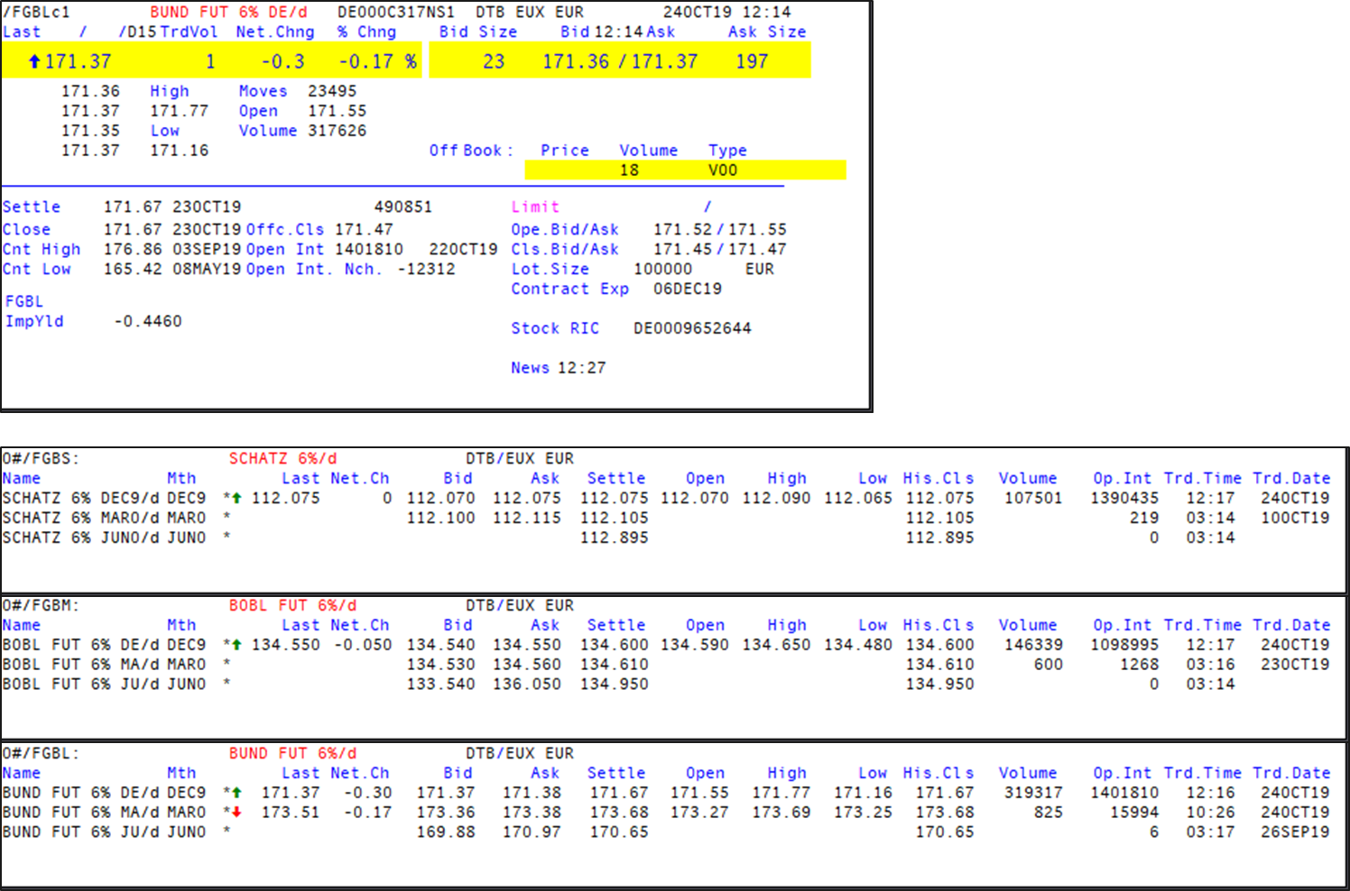
A clearing mechanism is a margining mechanism the involves one or more of:

Bund future specifications:
The ideal bond is not available, thus, we need a conversion factor $\text{CF}_{\text{Bond}}$
$$ \begin{align*} \text{CF}_{\text{Bond}} &= \frac{\text{PV}_{\text{Bond}}(@6\%)}{\text{PV}_{\text{Underlying}}(@6\%)}\\ &= \frac{\text{PV}_{\text{Bond}}(@6\%)}{100}. \end{align*} $$The conversion factor allows us to calculate the payment at deilvery
$$\text{Delivery payment} = \text{EDSP} \times \text{CF}_{\text{Bond}} \times 100,000 + \text{Accrued} $$"The final settlement price [EDSP] is established by Eurex on the final settlement day at 12:30 CET based on the volume-weighted average price of all trades during the final minute of trading provided that more than ten trades occurred during this minute; otherwise the volume-weighted average price of the last ten trades of the day, provided that these are not older than 30 minutes. If such a price cannot be determined, or does not reasonably reflect the prevailing market conditions, Eurex will establish the final settlement price." (Eurex Exchange 2019)
import calendar
from datetime import datetime
from dateutil.relativedelta import relativedelta

class Bond():
    def __init__(self, settlement:str, maturity:str, coupon:float=0):
        self.settlement = datetime.fromisoformat(settlement)
        self.maturity = datetime.fromisoformat(maturity)
        self.coupon = coupon
        if self.coupon > 0:
            # List of coupon payment days (ignoring modified following)
            self.coupon_shedule = [self.maturity]
            while True:
                coupon_date = min(self.coupon_shedule) - relativedelta(years=1)
                if coupon_date < self.settlement: break
                self.coupon_shedule.append(coupon_date)
            self.coupon_shedule.sort()
            # The next element in the coupon shedule (accrued interest)
            self.next_coupon = min(self.coupon_shedule)
            self.previous_coupon = min(self.coupon_shedule) - relativedelta(years=1)
            self.last_coupon = max(self.coupon_shedule)
            # Accrued interest
            self.accrued_period = self.actact(self.previous_coupon, self.settlement)
            self.accrued = self.coupon * self.accrued_period

    def actact(self, start_date:datetime, end_date:datetime):
        if start_date == end_date:
            return 0.0
        start_date = datetime.combine(start_date, datetime.min.time())
        end_date = datetime.combine(end_date, datetime.min.time())
        start_year = start_date.year
        end_year = end_date.year
        year_1_diff = 366 if calendar.isleap(start_year) else 365
        year_2_diff = 366 if calendar.isleap(end_year) else 365
        total_sum = end_year - start_year - 1
        diff_first = datetime(start_year + 1, 1, 1) - start_date
        total_sum += diff_first.days / year_1_diff
        diff_second = end_date - datetime(end_year, 1, 1)
        total_sum += diff_second.days / year_2_diff
        return total_sum

    def cleanprice(self, ytm:float=None):
        price = 0
        if self.coupon > 0:
            for t in bond.coupon_shedule:
                t_period = self.actact(self.settlement, t)
                price += self.coupon * 1 / (1 + ytm) ** t_period
            # Dirty price
            price += 100 / (1 + ytm) ** t_period
            # Clean price
            return price - self.accrued
        else:
            price += 100 / (1 + ytm) ** self.actact(self.settlement, self.maturity)
            return price

    def dirtyprice(self, ytm:float=None):
        if self.coupon > 0:
            return self.cleanprice(ytm) + self.accrued
        else:
            return self.cleanprice(ytm)

# Some bond
bond = Bond("2004-03-10", "2013-01-04", 4.5)
print(f"Accrued interest: EUR  {bond.accrued:.4f}")
print(f"Clean price @6%:  EUR {bond.cleanprice(0.06):.4f}")
# Another bond
bond_two = Bond("2004-03-10", "2013-01-04", 8.5)
print(f"Accrued interest: EUR  {bond_two.accrued:.4f} (another bond)")
print(f"Clean price @6%:  EUR {bond_two.cleanprice(0.06):.4f} (another bond)")
Accrued interest: EUR  0.8115
Clean price @6%:  EUR 89.9344
Accrued interest: EUR  1.5328 (another bond)
Clean price @6%:  EUR 116.7072 (another bond)
Now that we have the conversion factor ($\text{CF}_{\text{Bond}}$), we have to choose which bond to deliver at maturity. This is the cheapest-to-deliver, which can be identified by its implied repo rate
$$ \text{Implied repo} = \frac{\text{Delivery payment} - \text{Dirty price}}{\text{Dirty price} \times \frac{\text{Days to settlement}}{360}} $$A Repo trade is the agreement to sell (Spot) and buy back ($t+n$) an asset. Spot short and at the same time future long can be seen as a repo trade. Another interpretation is collateralized lending. The bond with the highest Implied Repo rate is the cheapest to deliver (CTD).
The forward price for the bond cheapest to deliver (CTD) is determined by the costs of acquiring the bond now and holding it until it shall be delivered to fulfil the obligation from the future. The cost of carry model applies, hence,
$$\text{Forward price} = \text{Spot price} + \text{Financing costs} - \text{Accrued income}$$Considering the underlying of the future,
$$\text{Theoretical future} = \frac{\text{Forward price}}{\text{CF}_{\text{Bond}}}$$Basis Point Value (BPV = PVO1) Hedge is a Nominal hedge, adjusted for underlying Basis Risk.
$$\text{Basis point hedge ratio} = \text{Simple hedge ratio} \times \text{CF}_{\text{CTD}} \times \frac{\text{BPV}_\text{Spot}}{\text{BPV}_\text{CTD}}$$PVO1 or BPV is the MTM change caused by a $0.0001$ = 1bp shift in yield.
Reading:
An option is a financial derivative contract that grants the holder (long position) the right, but not the obligation, to buy (call) or sell (put) an underlying asset at a predetermined price ($K$) within a specified time frame ($T$). The buyer pays a premium for this right, which is in contrast to the symmetric derivatives that we discussed before. Pricing (replicating) options is also more difficult than symmetric derivatives and requires the following assumptions:
Some relevant terminology:
Notation:
| Lower boundaries | Upper boundaries | |
|---|---|---|
| European Call | $c \ge S-K e^{-rT}$ | $c \le S$ |
| American Call | $C \ge S-Ke^{-rT}$ | $C \le S$ |
| European Put | $p \ge K e^{-rT} - S$ | $p \le K e^{-rT}$ |
| American Put | $P \ge K - S$ | $P \le K$ |
Why it makes no sense to execute an american call option prematurely, consider two portfolios A and B:
Consider random variable $X \sim \mathcal{N}(\mu,\sigma^2)$ as an example for an absolutely continuous univariate distribution.
Probability density function (PDF): $$\phi(x) = \frac{d\Phi(x)}{dx} = \frac{1}{\sigma \sqrt{2\pi}} e^{-\frac{1}{2} \left( \frac{x-\mu}{\sigma} \right)^2 }$$
Cumulative distribution function (CDF): $$\Phi(x) = P(X \le x) = \int_{-\infty}^x \phi(u)\; du$$
Quantile function, i.e. inverse of the CDF: $$\Phi^{-1}(p) = \inf \{x \in \mathbb{R}: p \le \Phi(x)\},\;\; p \in (0,1)$$
"""PDF vs CDF
"""
import matplotlib.pyplot as plt
import numpy as np
from scipy.stats import norm

x = np.linspace(-3, 3, 100)
p = np.linspace(0, 1)

fig_pdf = plt.figure("pdf")
plt.title("Probability Density Function (PDF)")
plt.plot(x, norm.pdf(x, 0, 1))
plt.plot(x, norm.pdf(x, 1, 1))
plt.plot(x, norm.pdf(x, 0, 1.5))
plt.axvline(x=-2.5, color='red', linewidth=.75)
plt.axvline(x=0, color='grey', linewidth=.75)
plt.legend(["N(0, 1)", "N(1, 1)", "N(0, 1.5)"], loc='upper left')
plt.close()

fig_cdf = plt.figure("cdf")
plt.title("Cumulative Distribution Function (CDF)")
plt.plot(x, norm.cdf(x, 0, 1))
plt.plot(x, norm.cdf(x, 1, 1))
plt.plot(x, norm.cdf(x, 0, 1.5))
plt.axvline(x=-2.5, color='red', linewidth=.75)
plt.axvline(x=0, color='grey', linewidth=.75)
plt.legend(["N(0, 1)", "N(1, 1)", "N(0, 1.5)"], loc='upper left')
plt.close()

fig_qf = plt.figure("qf")
plt.title("Quantile function (inverse CDF)")
plt.plot(p, norm.ppf(p, 0, 1))
plt.plot(p, norm.ppf(p, 1, 1))
plt.plot(p, norm.ppf(p, 0, 1.5))
plt.axvline(x=0.5, color='grey', linewidth=.75)
plt.legend(["N(0, 1)", "N(1, 1)", "N(0, 1.5)"], loc='upper left')
plt.close()
display(fig_pdf)

display(fig_cdf)

display(fig_qf)

In probability theory and statistics, the term Markov property refers to the memoryless property of a stochastic process, i.e. only the present price is relevant for predicting the future. Markov property is consistent with the weak form of market efficiency!
A stochastic process $X$, with drift $\mu$ and dispersion $\sigma$, follows a generalized Wiener process if it satisfies the following stochastic differential equation (SDE)
$$ dX_t = \mu \times dt + \sigma \times dW_t $$Note that by definition, the increments of a Wiener process are normally distributed. Specifically, for any $t > 0$,
$$ W_t - W_0 \sim \mathcal{N}(0, t) $$—that is, they are normally distributed with mean zero and variance $t$.
For an arbitrary initial value $X_0$:
$$ X_t = X_0 + \mu \times t + \sigma \times z \times \sqrt{t} $$where $z \sim \mathcal{N}(0, 1)$.
"""Calculate the probability of illiquidity
"""
import matplotlib.pyplot as plt
import numpy as np
from scipy.stats import norm

def prob_illiquid(m, const=2, drift=.1, variance=.16):
    expected_cash = const + drift * m
    sigma = (variance * m)**0.5
    p_illiquid = norm.cdf( (0 - expected_cash) / sigma ,0,1)  # normalization: (x - mu) / sigma
    return p_illiquid

X = range(1,12*5, 1)
fX = list(map(lambda m: prob_illiquid(m), X))

fig_illiquidity = plt.figure('Illiquidity', figsize=(9,4))
plt.title("Illiquidity")
plt.plot(X, fX)
plt.xlabel("Month (m)")
plt.ylabel("Probability")
plt.close()
display(fig_illiquidity)

A stochastic process $S$ follows a Geometric Brownian Motion (GBM) if it satisfies the following stochastic differential equation (SDE):
$$ dS_t = \mu S_t \, dt + \sigma S_t \, dW_t $$where $W_t$ is a Wiener process, i.e. a continuous-time stochastic process with normally distributed increments. Specifically, for any $t > 0$, the increment $W_t - W_0 \sim \mathcal{N}(0, t)$.
To derive the distribution and solution of the GBM, we apply Itô’s Lemma, which is the stochastic calculus analog of the chain rule. It allows us to compute the differential of a function of a stochastic process. See Itô, K. (1951). On stochastic differential equations (No. 4). American Mathematical Soc..
Let $S_t$ follow the SDE above, and define a new process $X_t = \ln S_t$. Then, by Itô’s Lemma:
$$ dX_t = \left( \frac{1}{S_t} \mu S_t - \frac{1}{2} \frac{1}{S_t^2} \sigma^2 S_t^2 \right) dt + \frac{1}{S_t} \sigma S_t \, dW_t = \left( \mu - \frac{\sigma^2}{2} \right) dt + \sigma \, dW_t $$Integrating both sides from $0$ to $t$ gives:
$$ X_t = X_0 + \left( \mu - \frac{\sigma^2}{2} \right)t + \sigma W_t $$Since $X_0 = \ln S_0$, we obtain the analytical solution:
$$ \ln S_t = \ln S_0 + \left( \mu - \frac{\sigma^2}{2} \right)t + \sigma W_t $$Exponentiating both sides yields the solution to the GBM:
$$ S_t = S_0 \exp\left( \left(\mu - \frac{\sigma^2}{2}\right) t + \sigma W_t \right) $$Therefore, we also have:
$$ \ln \frac{S_t}{S_0} = \left(\mu - \frac{\sigma^2}{2}\right) t + \sigma W_t $$Note that $W_t = z \sqrt{t}$ for $z \sim \mathcal{N}(0,1)$, which implies that $\ln \frac{S_t}{S_0}$ (log-return) is normally distributed, and $S_t$ is log-normally distributed.
from ipywidgets import interact, interactive, fixed, interact_manual
import ipywidgets as widgets
import numpy as np

import matplotlib.pyplot as plt
%matplotlib inline


#%% Create stock process:
# Random numbers N(0,1)
np.random.seed(888)
Z = np.random.normal(0, 1, 250)
def plot_gbm(mu, sigma):
    # returns for our geometric brownian motion
    R = Z * sigma * np.sqrt(1/250) + (mu-0.5*sigma**2) * 1/250
    # stock process (insert 100 for t=0)
    S = np.insert(100*np.exp(np.cumsum(R)), 0, 100)
    # Plotting
    plt.figure('GBM process', figsize=(9,4))
    plt.title(f"GBM ($\mu$ = {mu}, $\sigma$ = {sigma})")
    plt.axhline(y = 100, color ="black", linestyle ="--", linewidth=1)
    plt.plot(S)
    plt.xlabel("Time")
    plt.ylabel("Price")
    plt.ylim(30, 170)
    #plt.show()
interact(plot_gbm,
         mu = widgets.FloatSlider(value=0.1, min=-0.5, max=0.5, step=0.05),
         sigma = widgets.FloatSlider(value=0.25, min=0, max=0.9, step=0.05),
        )
interactive(children=(FloatSlider(value=0.1, description='mu', max=0.5, min=-0.5, step=0.05), FloatSlider(valu…
<function __main__.plot_gbm(mu, sigma)>
import numpy as np
import matplotlib.pyplot as plt
from scipy.stats import norm

S_0 = 50
mu = 0.16
sigma = 0.3

# Expected price and price volatility
S_1 = 50 * (1 + mu / 365)
print(f"E[S] tomorrow = {S_1:.4f}")
price_vola = 50 * sigma * (1 / 365)**0.5
print(f"Price vola    =  {price_vola:.4f}")

# Confidence interval
q975 = norm.ppf(0.975, 0, 1)
print(f"With 95% confidence: {S_1 - price_vola * q975 :.2f} < S_1 < {S_1 + price_vola * q975 :.2f}")

# Value at risk
q95 = norm.ppf(0.95, 0, 1)
print(f"1 day 95% VaR =  {S_0 * (sigma * (1 / 365)**0.5 * q95 - mu / 365) :.2f}")
E[S] tomorrow = 50.0219
Price vola    =  0.7851
With 95% confidence: 48.48 < S_1 < 51.56
1 day 95% VaR =  1.27
def gbm(mu, sigma, N=15):
    """Cumulative returns from a GBM
    """
    # Random numbers N(0,1)
    Z = np.random.normal(0, 1, N)
    # returns for our geometric brownian motion
    R = Z * sigma * np.sqrt(1/250) + (mu - 0.5*sigma**2) * 1/250
    # stock process (insert 100 for t=0)
    S = np.insert(np.exp(np.cumsum(R)), 0, 1)
    return S

fig_mc = plt.figure('MC', figsize=(9,4))
plt.title("Price path")
for n in range(100):
    plt.plot(S_0*gbm(mu, sigma), linewidth=2)
plt.xlabel("Trading days")
plt.ylabel("Price")
plt.close()
display(fig_mc)

"""Monte Caro simulation vs Black Scholes
"""
import numpy as np
from scipy.stats import norm
import matplotlib.pyplot as plt

# Option Parameters
S_0   = 220  # price of the underlying
K     = 220  # strike price
sigma = .98  # volatility
rate  = np.log(1.21)  # converting the ISDA rate to continous
T     = 1    # time to maturity

# We talk about this later, here its just a reference point
def black_scholes(cpflag,S,K,T,r,sigma):
    # cpflag in {1 for call, -1 for put}
    d1 = (np.log(S / K) + (r + 0.5 * sigma ** 2) * T) / (sigma * np.sqrt(T))
    d2 = (np.log(S / K) + (r - 0.5 * sigma ** 2) * T) / (sigma * np.sqrt(T))
    price = cpflag * (S * norm.cdf(cpflag*d1, 0.0, 1.0) - K * np.exp(-r * T) *
            norm.cdf(cpflag*d2, 0.0, 1.0))
    return price

print(f"The Black-Scholes (benchmark) price is: {black_scholes(1,220,220,1,np.log(1.21),0.98):,.2f}")
The Black-Scholes (benchmark) price is: 95.91
# Monte carlo pricing
def monte_carlo(cpflag,S,K,T,r,sigma,Nsim):
    Z = np.random.normal(0, 1, Nsim)
    S_T = S * np.exp(Z * sigma * np.sqrt(T) + (r-0.5*sigma**2) * T)
    CF_T = np.maximum(cpflag*(S_T - K),0)
    price = np.mean(CF_T) * np.exp(-r*T)
    return price

# Increase Nsim from 1000 to 100000 by 1000
X = range(1000,100000, 1000)
# Compute prices for all Nsim in X
mc_prices = list(map(lambda n: monte_carlo(1,220,220,1,np.log(1.21),0.98,n), X))

fig_mc_bs = plt.figure('Monte Caro simulation vs Black Scholes', figsize=(9,4))
plt.plot(X,mc_prices)
plt.axhline(y=black_scholes(1,220,220,1,np.log(1.21),0.98), color='orange')
plt.xlabel("Number of simulations")
plt.ylabel("Price of the option")
plt.legend(["Monte Carlo", "Black-Scholes"])
plt.close()
display(fig_mc_bs)

Reading:
Consider a replicating portfolio with bond (cash) $B$ and $\Delta$ share in the underlying asset $S$
$$ \begin{aligned} V_0 &= B + \Delta S_0\\ V_u &= B e^{rt} + \Delta S_u = (S_u - K)^+\\ V_d &= B e^{rt} + \Delta S_d = (S_d - K)^+ \end{aligned} $$Note that subtracting $V_d$ from $V_u$ yields
$$\Delta = \frac{(S_u - K)^+ - (S_d - K)^+}{S_u - S_d}$$"""Replicate the option payout in a one step lattice
"""
import numpy as np
# Weight of the underlying asset
def delta(flag, S_u, S_d, K): # flag = 1 (Call); -1 (Put)
delta = ( np.maximum(flag*(S_u - K), 0) - np.maximum(flag*(S_d - K), 0) ) / (S_u - S_d)
return delta
#print(delta(1, 60, 40, 45))
# Amount of bond in t = 0
def bond(flag, S_u, S_d, K, r, T):
beta = (np.maximum(flag*(S_u - K), 0) - delta(flag, S_u, S_d, K) * S_u) * np.exp(-r*T)
return beta
#print(beta(1, 60, 40, 45, 0.05, 1))
print(f"V_u = { bond(1, 60, 40, 45, 0.05, 1) * np.exp(.05) + delta(1, 60, 40, 45) * 60 :.0f}")
print(f"V_d = { bond(1, 60, 40, 45, 0.05, 1) * np.exp(.05) + delta(1, 60, 40, 45) * 40 :.0f}")
print(f"V_0 = { bond(1, 60, 40, 45, 0.05, 1) + delta(1, 60, 40, 45) * 50 :.4f}")
V_u = 15
V_d = -0
V_0 = 8.9631
The underlying of an option with maturity $T$ is modelled by an $n$ step binomial tree, with time between two steps of the tree $\Delta t = T / n$. With up move $u$ and down move $d$
$$u = \exp\left(\sigma \sqrt{\Delta t}\right)$$$$d = u^{-1}$$The following must hold for the up move probability $p$, in order to ensure martingale property,
$$S_0 = \left( S_0 \times u \times p + S_0 \times d \times (1-p) \right) e^{-r\Delta t} \implies p = \frac{e^{r\Delta t} - d}{u - d}$$Remember the binomial probability mass function (PMF)
$$f(k,n,p) = {n \choose k} p^k (1-p)^{n-k}$$here, $n$ is the number of steps in the tree and $k$ the number of up moves to reach a state $S_T$.
The CRR model is solved recuresively by discounting expected values. For American options, the buyer has the right to exercise at any point in time. Due to its discrete modelling of time, the CRR model allows execution at any node in the lattice. However, the buyer would only execute if the value that can be realized through execution $IV_t$ (intrinsic value) is above the discounted expected value of the next node. Therefore, the value that is considered for each node is
$$V_t = \max\left(E[V_{t+\Delta t}]e^{-r\Delta t}, IV_t \right).$$Solve recursively by stepwise discounting $V_t$ backwards in the tree. In this example we consider a European call with $S_0 = 220$, $K=165$, $\sigma = 98\%$, $T=1$, $r = 21\%$ ISDA.

"""Replicating options, Cox Ross Rubinstein style
"""
import numpy as np
import matplotlib.pyplot as plt

# INPUTS
S_0   = 220  # price of the underlying
K     = 220  # strike price
sigma = .98  # volatility
rate  = np.log(1.21)  # converting the ISDA rate
T     = 1    # time to maturity
steps = 2    # steps

# see Slide 10
dt = T / steps
u = np.exp(sigma * np.sqrt(dt))
d = 1 / u

fig_bintree = plt.figure('Binomial tree', figsize=(9,4))
binomial_tree = []
for n in range(steps+1):
    binomial_tree.append([])
    for k in range(n+1):
        S_nk = S_0 * u**(k) * d**(n-k)
        binomial_tree[-1].append(S_nk)
        plt.plot(n*dt, S_nk, 'ro')  # this will take forever for large # steps
        plt.annotate(f"{S_nk:.0f}  ", (n*dt, S_nk), ha='right', va='center')
print(binomial_tree)
plt.close()
[[220.0], [110.02008068234205, 439.9196919310029], [55.02008251522298, 220.0, 879.6787970394022]]
display(fig_bintree)
"""Full CRR model
"""
import matplotlib.pyplot as plt
import numpy as np

def Binomial(n, S, K, r, v, t, PutCall=1, American=False):
    At = t/n
    u = np.exp(v*np.sqrt(At))
    d = 1./u
    p = (np.exp(r*At)-d) / (u-d)
    # Binomial price tree
    stockvalue = np.zeros((n+1,n+1))
    stockvalue[0,0] = S
    for i in range(1,n+1):
        stockvalue[i,0] = stockvalue[i-1,0]*u
        for j in range(1,i+1):
            stockvalue[i,j] = stockvalue[i-1,j-1]*d
    # option value at final node
    optionvalue = np.zeros((n+1,n+1))
    for j in range(n+1):
        optionvalue[n,j] = max(0, PutCall*(stockvalue[n,j]-K))
    # recursive calculations
    for i in range(n-1,-1,-1):
        for j in range(i+1):
            if American:
                optionvalue[i,j] = max(0, PutCall*(stockvalue[i,j]-K), np.exp(-r*At)*(p*optionvalue[i+1,j]+(1-p)*optionvalue[i+1,j+1]))
            else:
                optionvalue[i,j] = np.exp(-r*At)*(p*optionvalue[i+1,j]+(1-p)*optionvalue[i+1,j+1])
    return optionvalue[0,0]
# Inputs
S_0   = 220  # price of the underlying
K     = 220  # strike price (165 vs 220)
sigma = .98  # volatility
rate  = np.log(1 + 0.21)  # converting the ISDA rate
T     = 1    # time to maturity
steps = 2    # steps

#Graphs and results for the Option prices
print("European Call Price: %s" %(Binomial(steps, S_0, K, rate, sigma, T, PutCall=1)))
print("American Call Price: %s" %(Binomial(steps, S_0, K, rate, sigma, T, PutCall=1, American=True)))
print("European Put  Price: %s" %(Binomial(steps, S_0, K, rate, sigma, T, PutCall=-1)))
print("American Put  Price: %s" %(Binomial(steps, S_0, K, rate, sigma, T, PutCall=-1, American=True)))
European Call Price: 87.25679654189224
American Call Price: 87.25679654189224
European Put  Price: 49.07497836007403
American Put  Price: 59.982962882003555
"""Spot price vs cash flow (put-call parity)
"""
import numpy as np
import matplotlib.pyplot as plt

# see workbook task 4 ff.
S_T = np.linspace(0,150)
K = 50

# portfolio
CF_CoN = K * (S_T > K)
CF_AoN = S_T * (S_T > K)
CF_T = CF_AoN - CF_CoN
# the rest is plotting
# hacky removal of 0 (looks better in plot)
CF_CoN = np.array(CF_CoN, dtype=np.double)
CF_CoN[CF_CoN==0] = np.nan
CF_AoN = np.array(CF_AoN, dtype=np.double)
CF_AoN[CF_AoN==0] = np.nan

fig_binpcp = plt.figure('PCP', figsize=(9,4))
plt.plot(S_T, CF_T, label="Call option")
plt.plot(S_T, CF_CoN, label="Cash or nothing")
plt.plot(S_T, CF_AoN, label="Asset or nothing")
plt.axhline(y=0, linewidth=1, color="black")
plt.xlabel("Spot price")
plt.ylabel("Cash flow")
plt.annotate("K", (K,-5))
plt.legend(loc="upper left")
plt.close()
display(fig_binpcp)

from scipy.stats import binom

# Recall our CRR parameters
sigma = .98  # volatility
rate  = np.log(1 + 0.21)  # converting the ISDA rate
T     = 1    # time to maturity
steps = 2    # steps
dt = T / steps
u = np.exp(sigma*np.sqrt(dt))
d = 1 / u
p = (np.exp(rate*dt)-d) / (u-d)
# Binary option cash flow calculations
CoN_payout = []
AoN_payout = []
for n, S in enumerate(binomial_tree[-1]):  # This is the binomial tree that we generated above
    if S > 165:  # strike
        AoN_payout.append( binom.pmf(n, steps, p) * S * np.exp(-rate*T) )
        CoN_payout.append( binom.pmf(n, steps, p) * 165 * np.exp(-rate*T) )
AoN = sum(AoN_payout)
CoN = sum(CoN_payout)
print(f"Price asset or nothing = {AoN:.4f}")
print(f"Price cash or nothing  =  {CoN:.4f}")
print(f"AoN - CoN              = {AoN - CoN:.4f}")
print(f"CRR call price (above) = {Binomial(steps, S_0, 165, rate, sigma, T, PutCall=1):.4f}")
Price asset or nothing = 203.6337
Price cash or nothing  =  87.2827
AoN - CoN              = 116.3510
CRR call price (above) = 116.3510
Consider the minimum return required to exercise the option
$$r_{min} = \ln\left(\frac{K}{S_0}\right)$$as well as the expected geometric return under the risk neutral measure (see the GBM introduced before)
$$E^\mathbb{Q}[r] = r \times T - \sigma^2 \frac{T}{2}$$Given the assumption of normally distributed log-returns, we have the standardization
$$ \begin{align*} d_{-} = d_{2} &= - \frac{\ln\left(\frac{K}{S_0}\right) - \left( r T - \sigma^2 \frac{T}{2} \right)}{\sigma \sqrt{T}}\\ &= \frac{\ln\left(\frac{S_0}{K}\right) + rT - \sigma^2 \frac{T}{2}}{\sigma \sqrt{T}} \end{align*} $$Which gives us the risk-neutral probability of exercising the option $N(d_-)$.
On the other hand you have $N(d_+)$ also known as $N(d_1)$, where
$$d_+ = d_1 = \frac{\ln\left(\frac{S_0}{K}\right) + rT + \sigma^2 \frac{T}{2}}{\sigma \sqrt{T}}$$$N(d_+)$ is also known as the delta of the option, i.e. the sensitivity of the option price towards a change in underlying $S_0$. Compare this to the $\Delta$ that we have already calculated for the binomial model above.
with
$$d_\pm = \frac{\ln\left(\frac{S_0}{K}\right) + rT \pm \sigma^2 \frac{T}{2}}{\sigma \sqrt{T}}$$with
$$d_\pm = \frac{\ln\left(\frac{S_0}{K}\right) + (r-q)T \pm \sigma^2 \frac{T}{2}}{\sigma \sqrt{T}}$$with
$$d_\pm = \frac{\ln\left(\frac{F_T}{K}\right) \pm \sigma^2 \frac{T}{2}}{\sigma \sqrt{T}}$$Black76 is useful whenerver there exists a liquid forward/futures market, e.g.:
Reading:
Let's quickly review the peculiarities of interest rate options, i.e.:
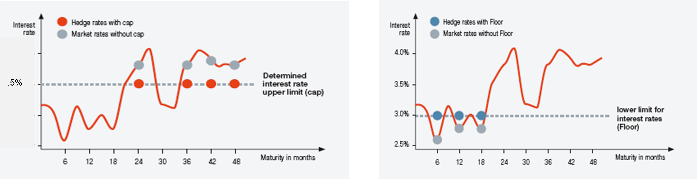
The interest cap (floor) offers an optional hedge against an increase (decrease) in the money market rate (EURIBOR, LIBOR, etc.), i.e. the hedging of an upper (lower) limit.
Caps (floors) consist of a strip of so-called "caplets" ("floorlets"), which are individual options on a strip of forward rates.
As an example, let us consider a interest cap (floor) with a term of 5 years against 6-month EURIBOR
Swaptions on the other hand simply represent the right to enter into a payer (receiver) swap, i.e. payer(/receiver)-swaption. The underling is therefore a forward swap.
import numpy as np
from scipy.stats import norm

#%% Black-Scholes formula
def black_scholes(cpflag,S,K,T,r,sigma):
    # cpflag in {1 for call, -1 for put}
    d1 = (np.log(S / K) + (r + 0.5 * sigma ** 2) * T) / (sigma * np.sqrt(T))
    d2 = (np.log(S / K) + (r - 0.5 * sigma ** 2) * T) / (sigma * np.sqrt(T))
    price = cpflag * (S * norm.cdf(cpflag*d1, 0.0, 1.0) - K * np.exp(-r * T) *
            norm.cdf(cpflag*d2, 0.0, 1.0))
    return price

print("European Call Price: %s" %(black_scholes(1,220,220,1,np.log(1.21),.98)))
print("European put  Price: %s" %(black_scholes(-1,220,220,1,np.log(1.21),.98)))
European Call Price: 95.91455141466928
European put  Price: 57.73273323285109
from ipywidgets import interact, interactive, fixed, interact_manual
import ipywidgets as widgets

import matplotlib.pyplot as plt
%matplotlib inline

def plot_block_scholes(pcflag, sigma, r, T):
    # Initial parameters
    X = np.linspace(1,100,100)
    plt.figure('BSM Price', figsize=(9,4))
    plt.plot(X,np.maximum(pcflag*(X-50),0), '--')
    plt.plot(X,black_scholes(pcflag,X,50,1,0.05,0.25))
    plt.plot(X,black_scholes(pcflag,X,50,T,r,sigma))
    plt.legend(["Intrinsic value", "Initial parameters", "Modified parameters"])
    plt.show()
    return None
interact(plot_block_scholes,
         pcflag=widgets.FloatSlider(value=1, min=-1, max=1, step=2),
         sigma=widgets.FloatSlider(value=0.25, min=0.1, max=0.5, step=0.05),
         r=widgets.FloatSlider(value=0.05, min=0.01, max=0.1, step=0.01),
         T=widgets.FloatSlider(value=1, min=0.5, max=5, step=0.5)
        );
interactive(children=(FloatSlider(value=1.0, description='pcflag', max=1.0, min=-1.0, step=2.0), FloatSlider(v…
"""CRR vs Black Scholes
"""
print(f"European Call Price: {black_scholes(1,220,220,1,np.log(1.21),.98):,.4f}")
print(f"European put  Price: {black_scholes(-1,220,220,1,np.log(1.21),.98):,.4f}")

X = range(2,100, 1)
crr_prices = list(map(lambda n: Binomial(n, 220, 220, np.log(1.21), .98, 1, PutCall=1), X))

fig_crr_bs = plt.figure('CRR vs Black Scholes', figsize=(9,4))
plt.plot(X,crr_prices)
plt.axhline(y=black_scholes(1,220,220,1,np.log(1.21),.98), color='orange')
plt.xlabel("Number of steps in the tree")
plt.ylabel("Price of the option")
plt.legend(["Cox-Ross-Rubinstein", "Black-Scholes"])
plt.close()
European Call Price: 95.9146
European put  Price: 57.7327
display(fig_crr_bs)

The European call price is simply the discounted expected value of its payout $E^\mathbb{Q}[(S_T - K)^+] e^{-rT}$, with
$$\begin{align} E^\mathbb{Q}[(S_T - K)^+] &= \int_K^\infty (S_T - K) f(S_T) dS_T\\ &=\int_K^\infty S_T f(S_T) dS_T - K \int_K^\infty f(S_T) dS_T \end{align}$$The terminal stock price at time $T$, under the risk-neutral measure, follows a log-normal distribution with $\mu = \ln S_0 + (r_f-\sigma^2 / 2)T$, variance $s^2 = \sigma^2 T$ and PDF
$$f(x) = \frac{1}{x s \sqrt{2 \pi}} \exp\left( -\frac{(\ln x - \mu)^2}{2 s^2} \right) $$Consider a contract where you receive the underlying $S_T$ conditional on $S_T > K$, note that this is different from a call option where the cash flow is $S_T - K$ under the condition that $S_T > K$. The price of this (expensive) option is $E^\mathbb{Q}[S_T 1_{\{S_T > K\}}] e^{-rT}$, where
$$E^\mathbb{Q}[S_T 1_{\{S_T > K\}}] = \int_K^\infty S_T f(S_T) dS_T$$Now consider an option that pays some amount $K$ (cash) conditional on $S_T > K$. The price of this (again expensive) option is $K \times P^\mathbb{Q}[S_T > K] e^{-rT}$, where
$$P^\mathbb{Q}[S_T > K] = \int_K^\infty f(S_T) dS_T$$Therefore, a European call option is a portfolio out of a long asset-or-noting option and a short cash-or-nothing option.
"""Straightforward integration vs Black Scholes
"""
import numpy as np
from scipy.stats import norm
from scipy.integrate import quad
import matplotlib.pyplot as plt

# See Chapter 2.4
def black_scholes(cpflag,S,K,T,r,sigma):
    # cpflag in {1 for call, -1 for put}
    d1 = (np.log(S / K) + (r + 0.5 * sigma ** 2) * T) / (sigma * np.sqrt(T))
    d2 = (np.log(S / K) + (r - 0.5 * sigma ** 2) * T) / (sigma * np.sqrt(T))
    price = cpflag * (S * norm.cdf(cpflag*d1, 0.0, 1.0) - K * np.exp(-r * T) *
            norm.cdf(cpflag*d2, 0.0, 1.0))
    return price

# probability density function P(S_T > K)
def PdF(S, S_0, rf, sd, t):
    A = 1 / ( np.sqrt(2*np.pi*t)*sd*S)
    B = np.exp(-(np.log(S)-(np.log(S_0)+(rf-0.5*sd**2)*t))**2/(2*sd**2*t))
    return A * B

# expected value S_T
def EdF(S, S_0, rf, sd, t):
    A = 1 / ( np.sqrt(2*np.pi*t)*sd*S)
    B = np.exp(-(np.log(S)-(np.log(S_0)+(rf-0.5*sd**2)*t))**2/(2*sd**2*t))
    return S * A * B

# expected value of (S_T - K)
def E2dF(S, S_0, rf, sd, t, K):
    A = 1 / ( np.sqrt(2*np.pi*t)*sd*S)
    B = np.exp(-(np.log(S)-(np.log(S_0)+(rf-0.5*sd**2)*t))**2/(2*sd**2*t))
    return (S - K) * A * B
# Inputs
S_0   = 220  # price of the underlying
K     = 220  # strike price
sigma = .98  # volatility
rate  = np.log(1.21)  # converting the ISDA rate
T     = 1    # time to maturity
steps = 2    # steps

# asset or nothin
AoN = quad(lambda x: EdF(x, S_0, rate, sigma, T), K, +np.inf)[0] * np.exp(-rate*T)
# cash or nothing with cash = K
CoN = K * quad(lambda x: PdF(x, S_0, rate, sigma, T), K, +np.inf)[0] * np.exp(-rate*T)
# straight forward integration
Call = quad(lambda x: E2dF(x, S_0, rate, sigma, T, K), K, +np.inf)[0] * np.exp(-rate*T)

print(f"Black-Scholes price        : {black_scholes(1,S_0,K,T,rate,sigma):.8f}")
print(f"AoN - CoN                  : {AoN-CoN:.8f}")
print(f"Straightforward integration: {Call:.8f}")
Black-Scholes price        : 95.91455141
AoN - CoN                  : 95.91455141
Straightforward integration: 95.91455141
# Just some plotting
x = np.linspace(1, 800, 100)
fig_bs_int, ax1 = plt.subplots(figsize=(9,4))
ax1.plot(x, PdF(x, S_0, rate, sigma, T))
ax1.set_xlabel('S_T')
ax2 = ax1.twinx()
ax2.plot(x, np.maximum(x-K,0), '--', color="black")
ax2.set_ylabel('max(S_T - K, 0)')
plt.close()
display(fig_bs_int)

Reading:
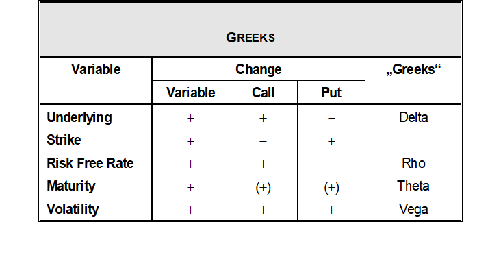
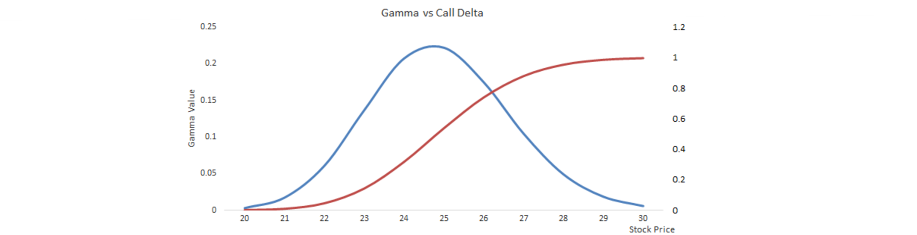
Greeks are partial derivatives that describe the sensitivity of the price of an option to a change in the respective underlying parameters.
Greeks are not constant, see e.g. delta (red) and gamma (blue)
Reading:
All parameters that determine the option price in a BSM model are observable, except $\sigma$. However, option prices are not calculated, they are the result of supply and demand on a liquid market. Thus, given an option price, we can find the $\sigma$ that ceteris paribus equates the BSM price with the market price.
"""Calculate implied volatility
"""
# Inputs
S_0   = 220  # price of the underlying
K     = 220  # strike price
rate  = np.log(1.21)  # converting the ISDA rate
T     = 1    # time to maturity
P_MKT = 85   # market price of the option

def iv_solve(IV):
    P_BSM = black_scholes(1,S_0,K,T,rate,IV)
    return (P_BSM - P_MKT)**2
IV = minimize(iv_solve, x0=0.25, bounds = ((0, None),)).x[0]

print(f'Implied vol: {IV:.4f}')
print(f'BSM price  : {black_scholes(1,S_0,K,T,rate,IV):.4f}')
Implied vol: 0.8251
BSM price  : 85.0000
Consider a matrix of option prices for different strikes and maturities. According to the theory, the resulting volatility surface should be flat, however, we usually observe sth like
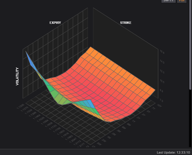
Reasons for a non-flat volatility surface
Risk adjusted discounting simply refers to using discount rates from a curve that appropriately represents the compensation for the credit worthiness of the obligor. The credit worthiness is often represented by a rating.
$$ \text{PV Bond} = \sum_{t=1}^T \frac{C_t}{(1 + r_{t, \text{Rating}})^t}. $$Instead of discounting with a risk adjusted discount rate, we can adjust the cash flows with their probability of being paid. Doing so requires additional information, namely:
Recovery rates (percentage values, rounded to two digits):
| Seniority | Recovery |
|---|---|
| Senior secured | 53.08 |
| Senior | 51.13 |
| Junior | 32.74 |
Cumulative default rates (percentage values, rounded to two digits):
| Rating | 1Y | 2Y | 3Y | 4Y | 5Y | 7Y | 10Y | 15Y |
|---|---|---|---|---|---|---|---|---|
| AAA | 0.00 | 0.00 | 0.07 | 0.15 | 0.24 | 0.66 | 1.40 | 1.40 |
| AA | 0.00 | 0.02 | 0.12 | 0.25 | 0.43 | 0.89 | 1.29 | 1.48 |
| A | 0.06 | 0.16 | 0.27 | 0.44 | 0.67 | 1.12 | 2.17 | 3.00 |
| BBB | 0.18 | 0.44 | 0.72 | 1.27 | 1.78 | 2.99 | 4.34 | 4.70 |
| BB | 1.06 | 3.48 | 6.12 | 8.68 | 10.97 | 14.46 | 17.73 | 19.91 |
| B | 5.20 | 11.00 | 15.95 | 19.40 | 21.88 | 25.14 | 29.02 | 30.65 |
| CCC | 19.79 | 26.92 | 31.63 | 35.97 | 40.15 | 42.64 | 45.10 | 45.10 |
The PV of the bond using risk adjusted cash flows, i.e. cash flows adjusted for the probability of their occurrence, is
$$ \text{PV Bond} = \sum_{t=1}^T \frac{C_t \times (1-p_t) + C_t \times \text{Recovery} \times p_t}{(1 + r_t)^t}, $$where $p_t$ is the cumulative probability up until time $t$.
A CDS contract works like an insurence that is linked to a credit event. This is, the protection buyer pays a premium $S$ (CDS spread) to the protection seller until the contract matures in $T$. In case of a default during the term of the contract, i.e. default in $\tau < T$, the protection buyer receives a settlement payment from the seller. This settlement payment is often, but not necessarily, designed to cover the loss given the default of a credit risky position, i.e. $(1 - \mathrm{Recovery})$.
Credit events (ISDA credit derivative definition 5/99 6/03 4/09 2/14):
What happens after a default? Lehman Brothers filed for bankruptcy on September 15, 2008. This marked the largest bankruptcy filing in U.S. history at the time. Here is the ISDA settlement timeline for Lehman Brothers:
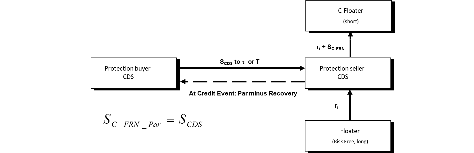
The payout can be replicarted with one credit risky and another risk free floater, which both trade at par. Shorting the risky floater yields 100% nominal, which can be invested into the risk free floater. The latter pays per definition the risk free rate $r_f$, wheres payments into the risky floater include an additional (credit) spread $r_f + S_{FRN = Par}$. In case of a credit event, the risk free floater is sold at 100%, whereas the risky floater is bought back at recovery. As this replicates the payout of the CDS $(1 - \mathrm{Recovery})$, the replicating credit spread must be equal to the CDS spread $S$. However, this is only an approximation, as it ignores that recovery is only paid on the nominal amount, transaction costs, and liquidity differences (availability) of the floaters.
$$S_{FRN = Par} \approx S$$If a floater is not trading at par, the replication does not work. However, the PV difference must be due to the discounted difference in spreads. Thus, given the spread $S_{FRN \neq Par}$ and price $P_{FRN\neq Par}$ of a non par floater, we can solve for the spread of the corresponding par floater $S_{FRN = Par}$
$$ \begin{align*} P_{FRN\neq Par} - 100\% &= PV(S_{FRN\neq Par} - S_{FRN = Par})\\ &= (S_{FRN\neq Par} - S_{FRN = Par}) \sum_{t=1}^T DF_t\\ &...\\ S_{FRN = Par} &= S_{FRN\neq Par} - \frac{P_{FRN \neq Par} - 100\%}{\sum_{t=1}^T DF_t} \end{align*} $$In reality, costs arise from shorting the FRN, i.e. the bond has to be borrowd for a fee $S_{Repo}$. Thus
$$S_{FRN = Par} + S_{Repo} = S$$No floater available? No problem, use an asset swap to create a synthetic floater, which at par is worth
$$ \begin{align*} 100\% &= P_\mathrm{Bond} - PV(C_\mathrm{Bond}) + PV(\mathrm{Libor} + S)\\\\ &= P_\mathrm{Bond} - C_\mathrm{Bond} \sum_{t=1}^T DF_t + 1 - DF_T + S \sum_{t=1}^T DF_t\\\\ S &= \frac{DF_T + C_\mathrm{Bond} \sum_{t=1}^T DF_t - P_\mathrm{Bond}}{\sum_{t=1}^T DF_t} \end{align*} $$If the bond is trading at par, $S$ is simply
$$S = C_\mathrm{Bond} - \frac{1-DF_T}{\sum_{t=1}^T DF_t}\\\\$$The asset swap spread is only an approximation for the CDS spread, as the CDS cash flow is not perfectly replicated (close out value of the swap) and there might be liquidity issues.
As always, the price of a financial product is the sum of its discounted (expected) cash flows. Accounting for credit risk simply means accounting for both, (risk free) interest rate and the probability of default.
Let $h_t$, the hazard rate (default intensity), be the probability to default in an infinitesimally short time interval $dt$.
$$h_t = \ln\left(\frac{1-p_{t-1}}{1-p_t} \right) \implies e^{h_t} = \frac{1-p_{t-1}}{1-p_t} \Longleftrightarrow p_t = 1 - \frac{1- p_{t-1}}{e^{h_t}}$$Then $a_t(h_t)$ is the present value of a paymment of $1$ at time $t$ if $t < \tau$, hence, no default. Think of this as a discount factor ($DF_t$) that also accounts for the likelyhood of the asset being alive.
$$a_t(h_t) = e^{-(h_t+r_t)t}$$On the other hand, $b_t(h_t)$ is the present value of a payment of 1 at time $t$ if $t-1 < \tau < t$, hence, default between $t-1$ and $t$.
$$b_t(h_t) = e^{-r_t t} \left( e^{-(h_t)t_{-1}} - e^{-(h_t)t} \right)$$Summing up the risky discount factors $a_t(h_t)$ and $b_t(h_t)$
$$ \begin{align*} A_T &= \sum_{t=1}^T a_t\\ B_T &= \sum_{t=1}^T b_t \end{align*} $$The fair CDS spread $S$ must fulfill
$$ \begin{align*} \text{PV Contingent leg} &= \text{PV Spead leg}\\ PV(1-\mathrm{Recovery}) &= PV(S)\\ B_T(1-\mathrm{Recovery}) &= A_T S \end{align*} $$and hence,
$$ S = \frac{B_T(1-\mathrm{Recovery})}{A_T} $$Hint: compare this to the single curve swap pricing above.
In practise, in preparation for central counterparty clearing, spread payments into a CDS are fixed at, i.e. $S^* \in \{0.002,0.01,0.05,0.1\}$, see ISDA agreements. Also the recovery rate is fixed, e.g. to 40% for investment grade. Therefore, contracts are unfair when entered and require an upfont payment
$$ \begin{aligned} \text{Upfront payment} &= B_T(1-\mathrm{Recovery}) - A_T S^*\\ &= (S - S^*) A_T \end{aligned} $$This is the upfront payment relative to the CDSs notional from the perspective of the protection buyer.
"""Fair spread and upfront payment
"""
import numpy as np

def CDS_AB(h, r, T):
    # assuming a constant hazard rate h
    A_T = 0
    B_T = 0
    for t in range(1, T+1):
        r_t = r[t-1] if isinstance(r, (list, np.ndarray)) else r
        A_T += np.exp(-(h + r_t)*t)
        B_T += np.exp(-r_t*t) * ( np.exp(-h*(t-1)) - np.exp(-h*t) )

    return (A_T, B_T)
# Example:
h = 0.005
R = 0.4

# Fair spread:
A_T, B_T = CDS_AB(h, 0.03, 1)
S = B_T*(1 - R) / A_T
print(f"Fair CDS spread: {S:.4f}")

# Upfront payment (spread payment of 100 basis points = 0.01)
upfront = (B_T*(1 - R) - A_T * 0.015) *1000000
upfront_alt = (S - 0.015) * A_T *1000000

print(f"Upfront payment on 10mln nominal: {upfront:.4f}")
print(f"Upfront payment on 10mln nominal: {upfront_alt:.4f}")
Fair CDS spread: 0.0030
Upfront payment on 10mln nominal: -11580.0109
Upfront payment on 10mln nominal: -11580.0109
Recall the CDS replication via floating rate notes, here we solve for $h$ in $A_T$ and $B_T$, using that $S_{FRN = Par} \approx S$
$$ \begin{align*} P_{FRN} - 100\% &= (S_{FRN} - S) A_T\\ &= A_T S_{FRN} - B_T(1-\mathrm{Recovery})\\ \end{align*} $$Note that for the par floater the problem simplifies to
$$\frac{S}{1-\mathrm{Recovery}} = \frac{B_T}{A_T} \approx h$$this is often called "credit triangle" and can be used as an approximation, even if the floater is not trading at par.
from scipy.optimize import minimize

r = 0.0917
T = 2
P_FRN = 1
S_FRN = 0.004
R = 0.2

def h_solve(h):
    A_T, B_T = CDS_AB(h, r, T)
    return (A_T*S_FRN - B_T*(1-R) + 1 - P_FRN)**2*100

# Find h that solves PV(alive) = PV(dead)
h = minimize(h_solve, x0=0.0001, bounds = ((0, None),)).x[0]

A_T, B_T = CDS_AB(h, r, T)
S = B_T*(1 - R) / A_T

print(f'Calibrated hazard rate: {h:.6f}')
print(f'Credit triangle       : {S_FRN/(1-R):.6f}')  # this works because P_FRN = 100% !
print(f'Calibrated CDS spread : {S:.6f}')
print(f'With A_T={A_T:.4f} and B_T={B_T:.6f}')
Calibrated hazard rate: 0.004988
Credit triangle       : 0.005000
Calibrated CDS spread : 0.004000
With A_T=1.7320 and B_T=0.008660
# This will convert the notebook to a html file
import os
# Convert to html slides
os.system('jupyter nbconvert derivatives.ipynb --to html')
0