Machine learning

Prof. Dr. Fabian Woebbeking

Assistant Professor of Financial Economics

IWH - Leibniz Institute for Economic Research,

MLU - Martin Luther University Halle-Wittenberg

fabian.woebbeking@iwh-halle.de

# Relevant imports
import os
import numpy as np
import pandas as pd
import openai
import numpy as np, matplotlib.pyplot as plt

Resources

Books:

• Müller and Guido. Introduction to machine learning with Python: a guide for data scientists.
• Hastie, Tibshirani and Friedman. The elements of statistical learning: data mining, inference, and prediction.
• Kuhn and Johnson. Applied predictive modeling.
• Hal Daumé III. A Course in Machine Learning (Free full text: http://ciml.info/)

Paper:

• Athey, S. "Beyond prediction: Using big data for policy problems." Science 355.6324 (2017): 483-485.
• Athey, S. The Impact of Machine Learning on Economics. The economics of artificial intelligence. University of Chicago Press, 2019. 507-552.
• Athey, S., and G. W. Imbens. Machine learning methods that economists should know about. Annual Review of Economics 11 (2019): 685-725.
• Mullainathan, S., and J. Spiess. Machine learning: an applied econometric approach. Journal of Economic Perspectives 31.2 (2017): 87-106.

ML in economic research

• Bajari, P., Nekipelov, D., Ryan, S. P., and M. Yang. Machine learning methods for demand estimation. American Economic Review 105.5 (2015): 481-85.
• Burgess, R., Hansen, M., Olken, B. A., and P. Potapov. The Political Economy of Deforestation in the Tropics. Quarterly Journal of Economics 127.4 (2012): 1707-54.
• Engl, F., Riedl, A., and R. Weber. Spillover Effects of Institutions on Cooperative Behavior, Preferences, and Beliefs. Amercian Economic Journal: Microeconomics 13.4 (2021): 261-99.
• Barth, A., Sasan M., and F. Woebbeking. "Let Me Get Back to You” - A Machine Learning Approach to Measuring NonAnswers. Management Science 69.10 (2023): 6333-6348.

Overview

• https://scikit-learn.org/stable/user_guide.html

Supervised learning

Some models: https://scikit-learn.org/stable/supervised_learning.html

Unsupervised

Some models: https://scikit-learn.org/stable/unsupervised_learning.html

Reinforcement learning

(Watch AlphaGo on Netflix, Prime, ...)

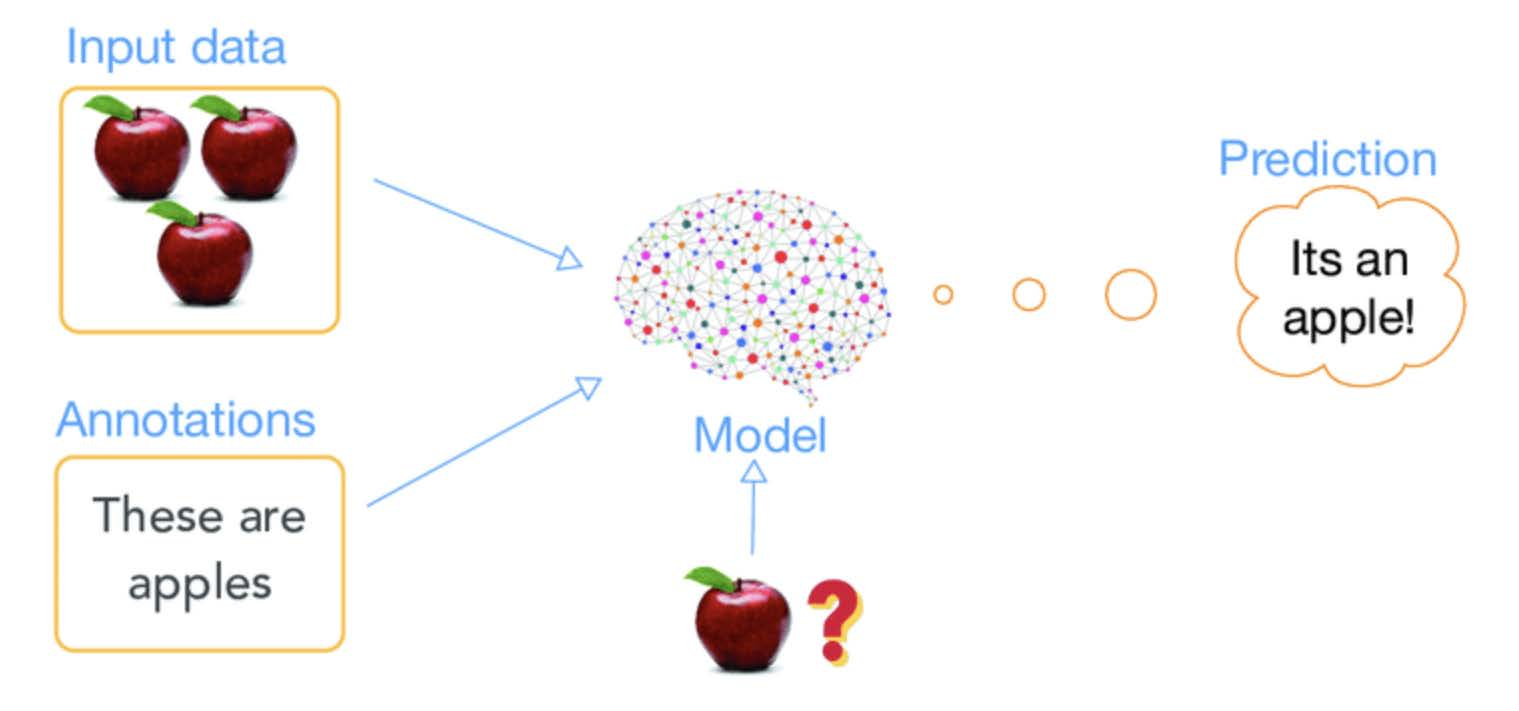
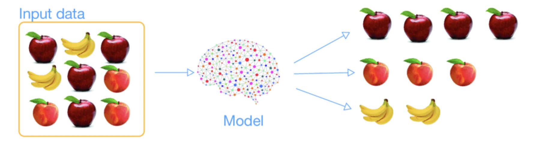
Universal approximation theorem

The universal approximation theorem states that a neural network with at least one hidden layer and a suitable activation function can approximate any continuous function on a compact domain, given sufficiently many neurons.

Therefore, this is not our problem:

def show_xsquared():
    x = np.linspace(-3, 3, 50)
    y = x**2
    
    plt.figure(figsize=(4, 3))
    plt.plot(x, y, label="y = x^2", color="blue")
    plt.title("y = x^2")
    plt.tight_layout()
    plt.show()

show_xsquared()

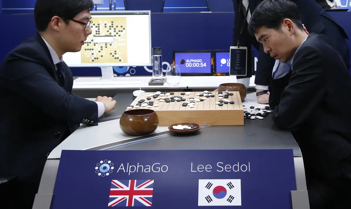
Selling your black box

• https://scikit-learn.org/stable/model_selection.html

• Athey, S. "Beyond prediction: Using big data for policy problems." Science 355.6324 (2017): 483-485.

Cross Validation

(Source: https://scikit-learn.org/stable/modules/cross_validation.html)

Explainable AI (XAI)

Various techniques aiming at

• Model interpretability (vs black box)
• Feature importance:
  • SHAP (SHapley Additive exPlanations)
  • LIME (Local Interpretable Model-agnostic Explanations)
• Visualization

Zoo of methods, e.g. LIME, Anchors, GraphLIME, LRP, DTD, PDA, TCAV, XGNN, SHAP, ASV, Break-Down, Shapley Flow, Textual Explanations of Visual Models, Integrated Gradients, Causal Models, Meaningful Perturbations, and X-NeSyL ... see:

• Holzinger, Andreas, et al. "Explainable AI methods-a brief overview." International Workshop on Extending Explainable AI Beyond Deep Models and Classifiers. Cham: Springer International Publishing, 2020.

Git(ing) ready

• http://rogerdudler.github.io/git-guide/

• https://guides.github.com/

• https://git-scm.com/book/en/v2

• https://peps.python.org/pep-0008/

Git and GitHub

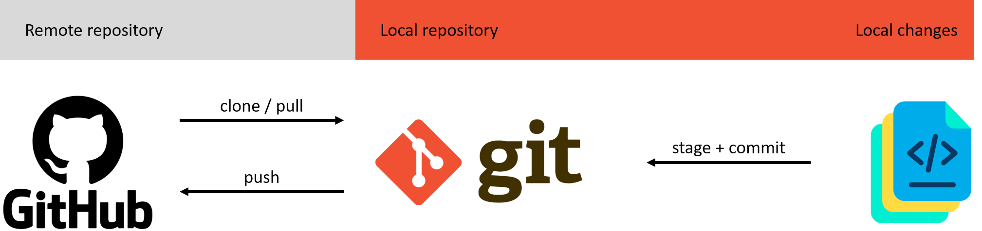
Git (local repository)

Git is a free and open source distributed version control system designed to handle everything from small to very large projects with speed and efficiency. (see Git, 2023)

Some source-code editors come with build-in Git (and even GitHub) capabilities or can be extended (e.g. Microsoft's Visual Studio Code, which I use during this course).

Your local repository is essentially a folder on your local file system. Changes made in that folder can be committed to the (local) git repository.

First, "stage" your changes - this is sth. like a pre-commit:

# The '*' adds all changes made in your local folder
git add *

Second, commit your staged changes to the local repository:

git commit -m 'Commit message'

In the broadest sense, you could see Git as a block chain of commits (changes) made to your repository. You can thus

• observe a complete (almost immutable) history.
• git checkout the state at any commit to the repository.

More on Git:

• About Git itself: https://git-scm.com/about
• Getting started (videos, tutorials): https://git-scm.com/doc

GitHub (remote repository)

You can clone the course repository to your local system:

git clone https://github.com/cafawo/MachineLearning.git

Your local Git repository remembers its origins. This enables you to pull updates from the remote (Git does not synchronize automatically).

git pull

If you have write access to the remote, you can also push changes to it.

git push

Careful: Git tries its best to merge the remote with the local repository, however, might fail if the two repositories are 'too' diverging. This should not concern you too much as a single user, but becomes very relevant when collaborating on a remote.

This is all we need for this course, however, it is only the tip of the iceberg. More on GitHub:

• Working with GitHub (remotes): https://skills.github.com/

Coding style

Without being too pedantic, we follow the PEP 8 – Style Guide for Python Code. When in doubt, return to this source for guidance.

Naming convention

Here are some best practices to follow when naming stuff.

• Use all lowercase. Ex: name instead of Name
• One exception: class names should start with a capital letter and follow by lowercase letters.
• Use snake_case convention (i.e., separate words by underscores, look like a snake). Ex: gross_profit instead of grossProfit or GrossProfit.
• Should be meaningful and easy to remember. Ex: interest_rate instead of r or ir.
• Should have a reasonable length. Ex: sales_apr instead of sales_data_for_april
• Avoid names of popular functions and modules. Ex: avoid print, math, or collections.

Comments

Comments should help to understand how your code works and your intentions behind it!

Comments that contradict the code are worse than no comments. Always make a priority of keeping the comments up-to-date when the code changes! Comments should be complete sentences. The first word should be capitalized, unless it is an identifier that begins with a lower case letter (never alter the case of identifiers!). (PEP 8)

Natural language processing (NLP)

How to squeeze textual data into machine learning methods?

Bag of words

Taddy, Matt. "Multinomial inverse regression for text analysis." Journal of the American Statistical Association 108.503 (2013): 755-770.

# Text input
malory = ["Do you want ants?",
          "Because that’s how you get ants."]

# All unique tokens from the text input (here words, could be n-grams)
feature_names = ['ants', 'because', 'do', 'get', 'how', 'that', 'want', 'you']

feature_matrix = np.array([[1, 0, 1, 0, 0, 0, 1, 1],
                           [1, 1, 0, 1, 1, 1, 0, 1]])

display(pd.DataFrame(feature_matrix, columns=feature_names, index=malory))

	ants	because	do	get	how	that	want	you
Do you want ants?	1	0	1	0	0	0	1	1
Because that’s how you get ants.	1	1	0	1	1	1	0	1

Word embedding

Mikolov, Tomas, et al. "Distributed representations of words and phrases and their compositionality." Advances in neural information processing systems 26 (2013).

Example: t-distributed Stochastic Neighbor Embedding (TSNE)

# Simplified word embeddings for cities and countries
word_embeddings = {
    "Paris": np.array([0.8, 0.2, 0.1]),
    "France": np.array([0.7, 0.2, 0.2]),
    "Berlin": np.array([0.6, 0.4, 0.2]),
    "Germany": np.array([0.6, 0.3, 0.3]),
    "Rome": np.array([0.5, 0.6, 0.2]),
    "Italy": np.array([0.5, 0.5, 0.3])
}

# Function to calculate cosine similarity between two vectors
def cosine_similarity(vec_a, vec_b):
    dot_product = np.dot(vec_a, vec_b)
    norm_a = np.linalg.norm(vec_a)
    norm_b = np.linalg.norm(vec_b)
    return dot_product / (norm_a * norm_b)

print(f"Paris|France: {cosine_similarity(word_embeddings['Paris'], word_embeddings['France']):.2f}")
print(f"Paris|Berlin: {cosine_similarity(word_embeddings['Paris'], word_embeddings['Berlin']):.2f}")
print(f"Paris|Italy:  {cosine_similarity(word_embeddings['Paris'], word_embeddings['Italy']):.2f}")

Paris|France: 0.99
Paris|Berlin: 0.93
Paris|Italy:  0.83

# Vector arithmetic: Berlin - Germany + France
result_vector = word_embeddings["Berlin"] - word_embeddings["Germany"] + word_embeddings["France"]

# Find the closest word to the resulting vector
closest_city = None
max_similarity = -1
for word in ["Paris", "Rome", "Italy"]: 
    similarity = cosine_similarity(result_vector, word_embeddings[word])
    if similarity > max_similarity:
        max_similarity = similarity
        closest_word = word

print(f"'Berlin' - 'Germany' + 'France' = '{closest_word}' ({similarity:.2f})")

'Berlin' - 'Germany' + 'France' = 'Paris' (0.90)

Transformer architecture

Vaswani, Ashish, et al. "Attention is all you need." Advances in neural information processing systems 30 (2017).

word_embeddings = {
    "Paris": np.array([0.8, 0.2, 0.1]),
    "France": np.array([0.7, 0.3, 0.2]),
    "Berlin": np.array([0.6, 0.1, 0.2]),
    "Germany": np.array([0.6, 0.4, 0.3]),
    "Rome": np.array([0.5, 0.2, 0.2]),
    "Italy": np.array([0.5, 0.5, 0.3])
    }

# This code is just illustrative ... look at the steps, not the code!
def transformer_encoder(word_embeddings):
    # Step 1: Input Embedding
    word_embeddings = word_embeddings

    # Step 2: Positional Encoding
    positional_embeddings = {word: vec + 0.1 for word, vec in word_embeddings.items()}

    # Step 3: Attention
    attention_sum = sum(positional_embeddings.values())
    attention_output = {word: vec * attention_sum for word, vec in positional_embeddings.items()}

    # Step 4: Feed-Forward Network
    feed_forward_output = {word: vec + np.array([0.3, 0.3, 0.3]) for word, vec in attention_output.items()}

    return feed_forward_output

Positional Encoding: This step modifies the original word embeddings by adding a positional value to each element. In real transformers, positional encoding is crucial because it provides information about the position of each word in the sequence. Our simple version just adds 0.1 to every element, but real models use more complex functions for positional encoding.

Attention: The self-attention mechanism in transformers allows each position in the encoder to consider every other position in the input sequence when computing its representation. In our example, we simulate self-attention by summing all the positional embeddings and then multiplying each embedding with this sum. This is a vast simplification and doesn't truly represent the selective attention mechanism used in real transformers.

Feed-Forward Network: In an actual transformer, each position's output from the self-attention layer is processed by a feed-forward neural network. This network consists of linear transformations and non-linear activations, allowing the model to learn complex transformations of the data. In our example, we simplify this by adding a fixed array [0.3, 0.3, 0.3] to each embedding vector, simulating a very basic transformation.

def classify_city_country(transformed_embeddings):
    classification = {}
    for word, vec in transformed_embeddings.items():
        # Classification rule: if the second element is greater than 1.2, classify as Country, else as City
        classification[word] = "Country" if vec[1] > 1.2 else "City"
    return classification


# Process the embeddings through the transformer encoder
transformed_embeddings = transformer_encoder(word_embeddings)

# Classify each word as City or Country
classification = classify_city_country(transformed_embeddings)

# Displaying the classification results
for word, category in classification.items():
    print(f"{word} is a {category}")

Paris is a City
France is a Country
Berlin is a City
Germany is a Country
Rome is a City
Italy is a Country

Fine tuning

• LLMs can be very large, hence, inefficient to train an LLM from scratch
• Fine tune the LLM to a specific task
  • Supervised learning process
  • Update weights of the LLM
• Check out: https://huggingface.co/

Catastrophic inference/forgetting

• Tendency of neural networks to forget previously learned information upon learning new information
• This creates a problem when updating a model on new data without retraining from scratch (e.g. when fine-tuning a fine-tuned model)
• Common solutions:
  • Regularization methods that penalize changes to important parameters
  • Rehearsal methods that store or generate examples from previous tasks
  • Dynamic architectures that grow or reconfigure network components

ChatGPT API

# Use your password to log in here ...
with open('gptpassword.txt', 'r') as file:
    openai.api_key = file.read().strip()

#returns a list of all OpenAI models
models = openai.models.list()
print(f"OpenAI currently offers {len(models.data)} models, e.g.:")
display(models.data[0:3])

OpenAI currently offers 48 models, e.g.:

[Model(id='gpt-4o-audio-preview-2024-10-01', created=1727389042, object='model', owned_by='system'),
 Model(id='gpt-4o-mini-audio-preview', created=1734387424, object='model', owned_by='system'),
 Model(id='gpt-4o-realtime-preview', created=1727659998, object='model', owned_by='system')]

Prompt engineering

messages = [{"role": "system", "content": 
    "You are a helpful assistant."}]
messages.append({"role": "user", "content": 
    "Classify into two categories, namely, 'City' and 'Country'"})
messages.append({"role": "user", "content": 
    "Classify this: Germany, Paris, France, Berlin, Rome, Italy"})
messages.append({"role": "user", "content": 
    "The output should be in JSON format."})

API call

# Send prompt to API and retrieve results
completion = openai.chat.completions.create(
                model="gpt-4", temperature=0.0, seed=2024, messages=messages
            )
print(completion.choices[0].message.content)

{
  "City": ["Paris", "Berlin", "Rome"],
  "Country": ["Germany", "France", "Italy"]
}

API parameters https://platform.openai.com/docs/api-reference

• temperature: "What sampling temperature to use, between 0 and 2. Lower values will make it more focused and deterministic."
• seed: "This feature is in Beta. If specified, our system will make a best effort to sample deterministically, such that repeated requests with the same seed and parameters should return the same result."

Many thanks and happy coding!

fabian.woebbeking@iwh-halle.de

# jupyter nbconvert vdt.ipynb --to slides --post serve --SlidesExporter.reveal_scroll=True
local_dir = %pwd
os.system(f'jupyter nbconvert {local_dir}/lecture.ipynb --to slides --SlidesExporter.reveal_scroll=True')

0

# Generate PDF
#os.system(f'jupyter nbconvert {local_dir}/ml.ipynb --to pdf')